Note
Go to the end to download the full example code.
Class 40 example#
This example shows how to define a composite lay-up with PyACP, solve the resulting model with PyMAPDL, and run a failure analysis with PyDPF Composites.
Begin with an MAPDL CDB file that contains the mesh, material data, and
boundary conditions. Import the file to PyACP to define the lay-up, and then export the
resulting model to PyMAPDL. Once the results are available, the RST file is loaded in
PyDPF Composites for postprocessing. The additional input files (material.xml
and ACPCompositeDefinitions.h5) can also be stored with PyACP and passed to PyDPF Composites.
The MAPDL and DPF services are run in Docker containers that share a volume (working directory).
Import modules and start ACP#
Import the standard library and third-party dependencies.
import os
import pathlib
import tempfile

import pyvista
Import the Ansys libraries.
import ansys.acp.core as pyacp
Launch the PyACP server and connect to it.
acp = pyacp.launch_acp()
Load mesh and materials from CDB file#
Define the directory in which the input files are stored.
try:
    EXAMPLES_DIR = pathlib.Path(os.environ["REPO_ROOT"]) / "examples"
except KeyError:
    EXAMPLES_DIR = pathlib.Path(__file__).parent
EXAMPLE_DATA_DIR = EXAMPLES_DIR / "data" / "class40"
Send class40.cdb to the server.
CDB_FILENAME = "class40.cdb"
local_file_path = str(EXAMPLE_DATA_DIR / CDB_FILENAME)
print(local_file_path)
cdb_file_path = acp.upload_file(local_path=local_file_path)
/home/runner/work/pyacp/pyacp/examples/data/class40/class40.cdb
Load the CDB file into PyACP and set the unit system.
model = acp.import_model(
    path=cdb_file_path, format="ansys:cdb", unit_system=pyacp.UnitSystemType.MPA
)
model
<Model with name 'ACP Lay-up Model'>
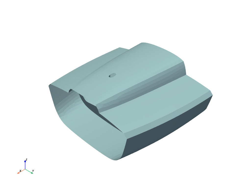
Visualize the loaded mesh.
Build Composite Lay-up#
Create the model (MPA unit system).
Materials#
mat_corecell_81kg = model.materials["1"]
mat_corecell_81kg.name = "Core Cell 81kg"
mat_corecell_81kg.ply_type = "isotropic_homogeneous_core"

mat_corecell_103kg = model.materials["2"]
mat_corecell_103kg.name = "Core Cell 103kg"
mat_corecell_103kg.ply_type = "isotropic_homogeneous_core"

mat_eglass_ud = model.materials["3"]
mat_eglass_ud.name = "E-Glass (uni-directional)"
mat_eglass_ud.ply_type = "regular"
Fabrics#
corecell_81kg_5mm = model.create_fabric(
    name="Corecell 81kg", thickness=0.005, material=mat_corecell_81kg
)
corecell_103kg_10mm = model.create_fabric(
    name="Corecell 103kg", thickness=0.01, material=mat_corecell_103kg
)
eglass_ud_02mm = model.create_fabric(name="eglass UD", thickness=0.0002, material=mat_eglass_ud)
Rosettes#
ros_deck = model.create_rosette(name="ros_deck", origin=(-5.9334, -0.0481, 1.693))
ros_hull = model.create_rosette(name="ros_hull", origin=(-5.3711, -0.0506, -0.2551))
ros_bulkhead = model.create_rosette(
    name="ros_bulkhead", origin=(-5.622, 0.0022, 0.0847), dir1=(0.0, 1.0, 0.0), dir2=(0.0, 0.0, 1.0)
)
ros_keeltower = model.create_rosette(
    name="ros_keeltower", origin=(-6.0699, -0.0502, 0.623), dir1=(0.0, 0.0, 1.0)
)
Oriented Selection Sets#
Note that the element sets are imported from the initial mesh (CBD file).
oss_deck = model.create_oriented_selection_set(
    name="oss_deck",
    orientation_point=(-5.3806, -0.0016, 1.6449),
    orientation_direction=(0.0, 0.0, -1.0),
    element_sets=[model.element_sets["DECK"]],
    rosettes=[ros_deck],
)

oss_hull = model.create_oriented_selection_set(
    name="oss_hull",
    orientation_point=(-5.12, 0.1949, -0.2487),
    orientation_direction=(0.0, 0.0, 1.0),
    element_sets=[model.element_sets["HULL_ALL"]],
    rosettes=[ros_hull],
)

oss_bulkhead = model.create_oriented_selection_set(
    name="oss_bulkhead",
    orientation_point=(-5.622, -0.0465, -0.094),
    orientation_direction=(1.0, 0.0, 0.0),
    element_sets=[model.element_sets["BULKHEAD_ALL"]],
    rosettes=[ros_bulkhead],
)

esets = [
    model.element_sets["KEELTOWER_AFT"],
    model.element_sets["KEELTOWER_FRONT"],
    model.element_sets["KEELTOWER_PORT"],
    model.element_sets["KEELTOWER_STB"],
]

oss_keeltower = model.create_oriented_selection_set(
    name="oss_keeltower",
    orientation_point=(-6.1019, 0.0001, 1.162),
    orientation_direction=(-1.0, 0.0, 0.0),
    element_sets=esets,
    rosettes=[ros_keeltower],
)
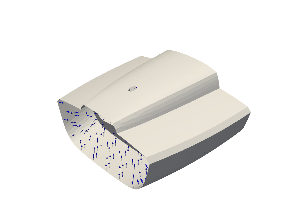
Show the orientations on the hull oriented selection set (OSS).
Note that the model must be updated before the orientations are available.
model.update()

plotter = pyvista.Plotter()
plotter.add_mesh(model.mesh.to_pyvista(), color="white")
orientation = oss_hull.elemental_data.orientation
assert orientation is not None
plotter.add_mesh(
    orientation.get_pyvista_glyphs(mesh=model.mesh, factor=0.2, culling_factor=5),
    color="blue",
)
plotter.show()
Modeling Plies#
Define plies for the hull, deck, and bulkhead.
angles = [-90.0, -60.0, -45.0 - 30.0, 0.0, 0.0, 30.0, 45.0, 60.0, 90.0]
for mg_name in ["hull", "deck", "bulkhead"]:
    mg = model.create_modeling_group(name=mg_name)
    oss_list = [model.oriented_selection_sets["oss_" + mg_name]]
    for angle in angles:
        add_ply(mg, "eglass_ud_02mm_" + str(angle), eglass_ud_02mm, angle, oss_list)
    add_ply(mg, "corecell_103kg_10mm", corecell_103kg_10mm, 0.0, oss_list)
    for angle in angles:
        add_ply(mg, "eglass_ud_02mm_" + str(angle), eglass_ud_02mm, angle, oss_list)
Add plies to the keeltower.
mg = model.create_modeling_group(name="keeltower")
oss_list = [model.oriented_selection_sets["oss_keeltower"]]
for angle in angles:
    add_ply(mg, "eglass_ud_02mm_" + str(angle), eglass_ud_02mm, angle, oss_list)

add_ply(mg, "corecell_81kg_5mm", corecell_81kg_5mm, 0.0, oss_list)

for angle in angles:
    add_ply(mg, "eglass_ud_02mm_" + str(angle), eglass_ud_02mm, angle, oss_list)
Inspect the number of modeling groups and plies.
print(len(model.modeling_groups))
print(len(model.modeling_groups["hull"].modeling_plies))
print(len(model.modeling_groups["deck"].modeling_plies))
print(len(model.modeling_groups["bulkhead"].modeling_plies))
print(len(model.modeling_groups["keeltower"].modeling_plies))
4
19
19
19
19
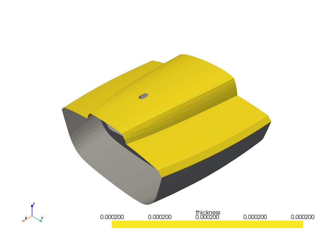
Show the thickness of one of the plies.
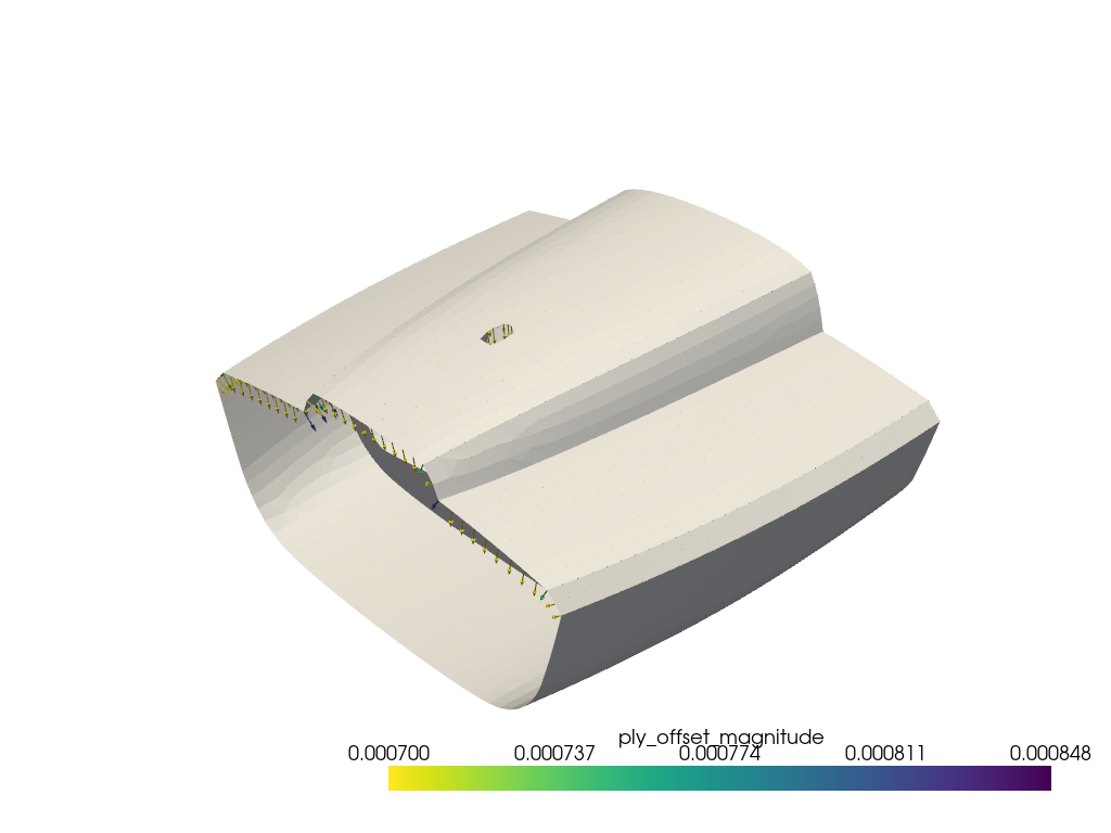
Show the ply offsets that are scaled by a factor of 200.
plotter = pyvista.Plotter()
plotter.add_mesh(model.mesh.to_pyvista(), color="white")
ply_offset = modeling_ply.nodal_data.ply_offset
assert ply_offset is not None
plotter.add_mesh(
    ply_offset.get_pyvista_glyphs(mesh=model.mesh, factor=200),
)
plotter.show()
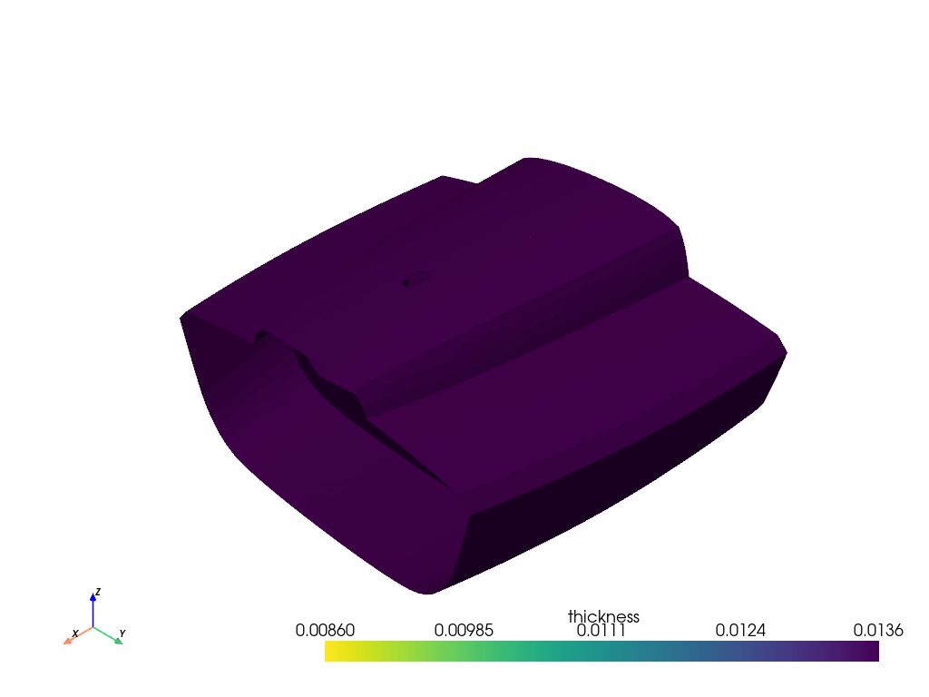
Show the thickness of the entire lay-up.
Write out ACP Model#
ACPH5_FILE = "class40.acph5"
CDB_FILENAME_OUT = "class40_analysis_model.cdb"
COMPOSITE_DEFINITIONS_H5 = "ACPCompositeDefinitions.h5"
MATML_FILE = "materials.xml"
Update and save the ACP model.
model.update()
model.save(ACPH5_FILE, save_cache=True)
Save the model as a CDB file for solving with PyMAPDL.
model.export_analysis_model(CDB_FILENAME_OUT)
# Export the shell lay-up and material file for PyDPF Composites.
model.export_shell_composite_definitions(COMPOSITE_DEFINITIONS_H5)
model.export_materials(MATML_FILE)
Download files from the ACP server to a local directory.
tmp_dir = tempfile.TemporaryDirectory()
WORKING_DIR = pathlib.Path(tmp_dir.name)
cdb_file_local_path = pathlib.Path(WORKING_DIR) / CDB_FILENAME_OUT
matml_file_local_path = pathlib.Path(WORKING_DIR) / MATML_FILE
composite_definitions_local_path = pathlib.Path(WORKING_DIR) / COMPOSITE_DEFINITIONS_H5
acp.download_file(remote_filename=CDB_FILENAME_OUT, local_path=str(cdb_file_local_path))
acp.download_file(remote_filename=MATML_FILE, local_path=str(matml_file_local_path))
acp.download_file(
    remote_filename=COMPOSITE_DEFINITIONS_H5, local_path=str(composite_definitions_local_path)
)
Solve with PyMAPDL#
Import PyMAPDL and connect to its server.
from ansys.mapdl.core import launch_mapdl

mapdl = launch_mapdl()
mapdl.clear()
Load the CDB file into PyMAPDL.
mapdl.input(str(cdb_file_local_path))
'\n /INPUT FILE= class40_analysis_model.cdb LINE= 0\n ANSYS RELEASE 11.0 UP20070125 16:39:41 03/10/2009\n\n *** MAPDL - ENGINEERING ANALYSIS SYSTEM RELEASE 24.2BETA ***\n Ansys Mechanical Enterprise \n 00000000 VERSION=LINUX x64 08:32:08 MAY 13, 2024 CP= 1.083\n\n \n\n\n\n ** WARNING: PRE-RELEASE VERSION OF MAPDL 24.2BETA\n ANSYS,INC TESTING IS NOT COMPLETE - CHECK RESULTS CAREFULLY **\n\n ***** MAPDL ANALYSIS DEFINITION (PREP7) *****\n\n\n ***** ROUTINE COMPLETED ***** CP = 1.148\n\n\n'
Solve the model.
mapdl.allsel()
mapdl.slashsolu()
mapdl.solve()
*****  MAPDL SOLVE    COMMAND  *****

 *** NOTE ***                            CP =       1.163   TIME= 08:32:08
 There is no title defined for this analysis.

 *** SELECTION OF ELEMENT TECHNOLOGIES FOR APPLICABLE ELEMENTS ***
                ---GIVE SUGGESTIONS ONLY---

 ELEMENT TYPE         1 IS SHELL181. IT IS ASSOCIATED WITH ELASTOPLASTIC
 MATERIALS ONLY. KEYOPT(8) IS ALREADY SET AS SUGGESTED. KEYOPT(3)=2
 IS SUGGESTED FOR HIGHER ACCURACY OF MEMBRANE STRESSES; OTHERWISE,
 KEYOPT(3)=0 IS SUGGESTED.

 ELEMENT TYPE         2 IS BEAM188 . KEYOPT(1)=1 IS SUGGESTED FOR NON-CIRCULAR CROSS
 SECTIONS AND KEYOPT(3)=2 IS ALWAYS SUGGESTED.

 ELEMENT TYPE         2 IS BEAM188 . KEYOPT(15) IS ALREADY SET AS SUGGESTED.

 ELEMENT TYPE         3 IS SHELL181. IT IS ASSOCIATED WITH ELASTOPLASTIC
 MATERIALS ONLY. KEYOPT(8) IS ALREADY SET AS SUGGESTED. KEYOPT(3)=2
 IS SUGGESTED FOR HIGHER ACCURACY OF MEMBRANE STRESSES; OTHERWISE,
 KEYOPT(3)=0 IS SUGGESTED.


 *** MAPDL - ENGINEERING ANALYSIS SYSTEM  RELEASE                  24.2BETA ***
 Ansys Mechanical Enterprise
 00000000  VERSION=LINUX x64     08:32:08  MAY 13, 2024 CP=      1.192


 ** WARNING: PRE-RELEASE VERSION OF MAPDL 24.2BETA
  ANSYS,INC TESTING IS NOT COMPLETE - CHECK RESULTS CAREFULLY **

                       S O L U T I O N   O P T I O N S

   PROBLEM DIMENSIONALITY. . . . . . . . . . . . .3-D
   DEGREES OF FREEDOM. . . . . . UX   UY   UZ   ROTX ROTY ROTZ
   ANALYSIS TYPE . . . . . . . . . . . . . . . . .STATIC (STEADY-STATE)
   GLOBALLY ASSEMBLED MATRIX . . . . . . . . . . .SYMMETRIC

 *** NOTE ***                            CP =       1.194   TIME= 08:32:08
 Poisson's ratio PR input has been converted to NU input.

 *** NOTE ***                            CP =       1.197   TIME= 08:32:08
 Present time 0 is less than or equal to the previous time.  Time will
 default to 1.

 *** NOTE ***                            CP =       1.198   TIME= 08:32:08
 The conditions for direct assembly have been met.  No .emat or .erot
 files will be produced.

                      L O A D   S T E P   O P T I O N S

   LOAD STEP NUMBER. . . . . . . . . . . . . . . .     1
   TIME AT END OF THE LOAD STEP. . . . . . . . . .  1.0000
   NUMBER OF SUBSTEPS. . . . . . . . . . . . . . .     1
   STEP CHANGE BOUNDARY CONDITIONS . . . . . . . .    NO
   COPY INTEGRATION POINT VALUES TO NODE . . . . .   YES
   PRINT OUTPUT CONTROLS . . . . . . . . . . . . .NO PRINTOUT
   DATABASE OUTPUT CONTROLS. . . . . . . . . . . .ALL DATA WRITTEN
                                                  FOR THE LAST SUBSTEP


 SOLUTION MONITORING INFO IS WRITTEN TO FILE= file.mntr

 *** NOTE ***                            CP =       1.261   TIME= 08:32:08
 Predictor is ON by default for structural elements with rotational
 degrees of freedom.  Use the PRED,OFF command to turn the predictor
 OFF if it adversely affects the convergence.


                         ***********  PRECISE MASS SUMMARY  ***********

   TOTAL RIGID BODY MASS MATRIX ABOUT ORIGIN
               Translational mass               |   Coupled translational/rotational mass
         324.96       0.46544E-18   0.14304E-17 |   -0.11582E-16    211.44      -0.36088E-02
        0.46544E-18    324.96      -0.49693E-17 |    -211.44      -0.96175E-17   -2015.3
        0.14304E-17  -0.49693E-17    324.96     |    0.36088E-02    2015.3       0.20783E-16
     ------------------------------------------ | ------------------------------------------
                                                |         Rotational mass (inertia)
                                                |     759.66       0.20436E-01    1316.9
                                                |    0.20436E-01    13054.      -0.32469E-02
                                                |     1316.9      -0.32469E-02    13218.

   TOTAL MASS =  324.96
     The mass principal axes coincide with the global Cartesian axes

   CENTER OF MASS (X,Y,Z)=   -6.2017       0.11105E-04   0.65067

   TOTAL INERTIA ABOUT CENTER OF MASS
         622.08      -0.19444E-02    5.6093
       -0.19444E-02    418.20      -0.89877E-03
         5.6093      -0.89877E-03    719.59

   PRINCIPAL INERTIAS =    621.76        418.20        719.92
   ORIENTATION VECTORS OF THE INERTIA PRINCIPAL AXES IN GLOBAL CARTESIAN
     ( 0.998,-0.000,-0.057) ( 0.000, 1.000, 0.000) ( 0.057,-0.000, 0.998)


  *** MASS SUMMARY BY ELEMENT TYPE ***

  TYPE      MASS
     1   322.570
     2   1.65744
     3  0.729815

 Range of element maximum matrix coefficients in global coordinates
 Maximum = 104467551 at element 771.
 Minimum = 31671440.9 at element 4058.

   *** ELEMENT MATRIX FORMULATION TIMES
     TYPE    NUMBER   ENAME      TOTAL CP  AVE CP

        1      3973  SHELL181      2.200   0.000554
        2        88  BEAM188       0.004   0.000049
        3        22  SHELL181      0.004   0.000183
 Time at end of element matrix formulation CP = 3.487432.

 SPARSE MATRIX DIRECT SOLVER.
  Number of equations =       24096,    Maximum wavefront =     66


  Memory allocated on this process
  -------------------------------------------------------------------
  Equation solver memory allocated                     =    66.685 MB
  Equation solver memory required for in-core mode     =    64.079 MB
  Equation solver memory required for out-of-core mode =    29.738 MB
  Total (solver and non-solver) memory allocated       =   670.556 MB

 *** NOTE ***                            CP =       3.534   TIME= 08:32:10
 The Sparse Matrix Solver is currently running in the in-core memory
 mode.  This memory mode uses the most amount of memory in order to
 avoid using the hard drive as much as possible, which most often
 results in the fastest solution time.  This mode is recommended if
 enough physical memory is present to accommodate all of the solver
 data.
 Sparse solver maximum pivot= 266668835 at node 2542 UY.
 Sparse solver minimum pivot= 1.78586102 at node 586 ROTZ.
 Sparse solver minimum pivot in absolute value= 1.78586102 at node 586
 ROTZ.

   *** ELEMENT RESULT CALCULATION TIMES
     TYPE    NUMBER   ENAME      TOTAL CP  AVE CP

        1      3973  SHELL181      4.911   0.001236
        2        88  BEAM188       0.009   0.000102
        3        22  SHELL181      0.007   0.000313

   *** NODAL LOAD CALCULATION TIMES
     TYPE    NUMBER   ENAME      TOTAL CP  AVE CP

        1      3973  SHELL181      0.055   0.000014
        2        88  BEAM188       0.001   0.000016
        3        22  SHELL181      0.000   0.000014
 *** LOAD STEP     1   SUBSTEP     1  COMPLETED.    CUM ITER =      1
 *** TIME =   1.00000         TIME INC =   1.00000      NEW TRIANG MATRIX


 *** MAPDL BINARY FILE STATISTICS
  BUFFER SIZE USED= 16384
        8.562 MB WRITTEN ON ASSEMBLED MATRIX FILE: file.full
       58.125 MB WRITTEN ON RESULTS FILE: file.rst
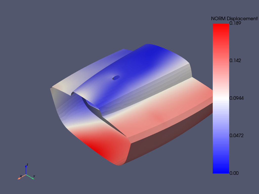
Show the displacements in postprocessing.
mapdl.post1()
mapdl.set("last")
mapdl.post_processing.plot_nodal_displacement(component="NORM")

# Download the RST file for further postprocessing.
rstfile_name = f"{mapdl.jobname}.rst"
rst_file_local_path = pathlib.Path(tmp_dir.name) / rstfile_name
mapdl.download(rstfile_name, tmp_dir.name)
['file.rst']
Postprocessing with PyDPF Composites#
To postprocess the results, you must configure the imports, connect to the PyDPF Composites server, and load its plugin.
from ansys.dpf.composites.composite_model import CompositeModel
from ansys.dpf.composites.constants import FailureOutput
from ansys.dpf.composites.data_sources import (
    CompositeDefinitionFiles,
    ContinuousFiberCompositesFiles,
)
from ansys.dpf.composites.failure_criteria import (
    CombinedFailureCriterion,
    CoreFailureCriterion,
    MaxStrainCriterion,
    MaxStressCriterion,
)
from ansys.dpf.composites.server_helpers import connect_to_or_start_server
from ansys.dpf.core.unit_system import unit_systems
Connect to the server. The connect_to_or_start_server function
automatically loads the composites plugin.
dpf_server = connect_to_or_start_server()
Specify the combined failure criterion.
max_strain = MaxStrainCriterion()
max_stress = MaxStressCriterion()
core_failure = CoreFailureCriterion()

cfc = CombinedFailureCriterion(
    name="Combined Failure Criterion",
    failure_criteria=[max_strain, max_stress, core_failure],
)
Create the composite model and configure its input.
composite_model = CompositeModel(
    composite_files=ContinuousFiberCompositesFiles(
        rst=rst_file_local_path,
        composite={
            "shell": CompositeDefinitionFiles(definition=composite_definitions_local_path),
        },
        engineering_data=matml_file_local_path,
    ),
    default_unit_system=unit_systems.solver_nmm,
    server=dpf_server,
)
Evaluate the failure criteria.
output_all_elements = composite_model.evaluate_failure_criteria(cfc)
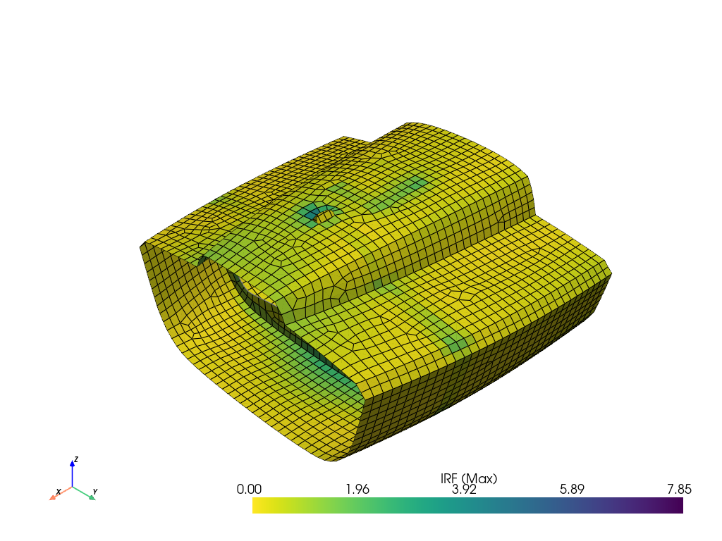
Query and plot the results.
irf_field = output_all_elements.get_field({"failure_label": FailureOutput.FAILURE_VALUE})
irf_field.plot()
Total running time of the script: (0 minutes 21.393 seconds)