Note
Go to the end to download the full example code.
Optimization example#
This example demonstrates how to use the ACP, MAPDL, and DPF servers to optimize the ply angles in a composite lay-up. The optimization aims to minimize the maximum inverse reserve factor (IRF) of the composite structure under two load cases.
The example uses the scipy.optimize.minimize() function to perform the optimization.
While the procedure itself is not the focus of this example and could be improved,
it demonstrates the process of optimizing a composite lay-up with PyACP.
Import modules and setup#
To setup the environment for this optimization example, you must perform these steps which are covered in the subsequent example code:
Import the required libraries.
Launch the ACP, MAPDL, and DPF servers.
Create a temporary directory to store the input and output files.
Import the standard library and third-party dependencies.
Import Ansys libraries
import ansys.acp.core as pyacp
import ansys.dpf.composites as pydpf_composites
import ansys.mapdl.core as pymapdl
Launch the PyACP server.
acp_instance = pyacp.launch_acp()
acp_instance.clear()
Launch the MAPDL server.
mapdl = pymapdl.launch_mapdl()
Launch the DPF server.
dpf_server = pydpf_composites.server_helpers.connect_to_or_start_server()
Create a temporary directory to store the input and output files.
Prepare the ACP model#
This example uses the optimization_model.dat file, which contains a simple ACP model
of a rounded square tube.
The prepare_acp_model function imports the optimization_model.dat file into a new
ACP model and creates a lay-up with six plies.
It returns a ACPWorkflow object that can be used to access the model and
generate the output files.
input_file = pyacp.example_helpers.get_example_file(
    example_key=pyacp.example_helpers.ExampleKeys.OPTIMIZATION_EXAMPLE_DAT,
    working_directory=workdir,
)


def prepare_acp_model(*, acp, workdir, input_file):
    # Import the DAT input file into a new ACP model
    acp_workflow = pyacp.ACPWorkflow.from_cdb_or_dat_file(
        acp=acp,
        cdb_or_dat_file_path=input_file,
        local_working_directory=workdir,
    )
    model = acp_workflow.model
    model.name = "optimization_example"

    element_set = model.element_sets["All_Elements"]
    material = model.create_material(
        name="Epoxy_Carbon_Woven_230GPa_Prepreg",
        ply_type=pyacp.PlyType.WOVEN,
        engineering_constants=(
            pyacp.material_property_sets.ConstantEngineeringConstants.from_orthotropic_constants(
                E1=6.134e10,
                E2=6.134e10,
                E3=6.9e9,
                nu12=0.04,
                nu23=0.3,
                nu13=0.3,
                G12=1.95e10,
                G23=2.7e9,
                G31=2.7e9,
            )
        ),
        stress_limits=(
            pyacp.material_property_sets.ConstantStressLimits.from_orthotropic_constants(
                Xt=8.05e8,
                Yt=8.05e8,
                Zt=5.0e7,
                Xc=-5.09e8,
                Yc=-5.09e8,
                Zc=-1.7e8,
                Sxy=1.25e8,
                Syz=6.5e7,
                Sxz=6.5e7,
            )
        ),
    )
    fabric = model.create_fabric(
        material=material,
        thickness=0.000254,  # 0.01 in
        name="Epoxy_Carbon_Woven_230GPa_Prepreg_0.01in",
    )
    rosette = model.create_rosette(
        origin=(0.0026, 0.0000, 0.0119),
        dir1=(0.0, 0.0, -1.0),
        dir2=(1.0, 0.0, 0.0),
    )
    oss = model.create_oriented_selection_set(
        element_sets=[element_set],
        orientation_point=(0.0021, 0.0, 0.0111),
        orientation_direction=(0, -1, 0),
        rosette_selection_method=pyacp.RosetteSelectionMethod.MINIMUM_ANGLE,
        rosettes=[rosette],
    )

    modeling_group = model.create_modeling_group(name="Modeling_Group")

    for _ in range(6):
        modeling_group.create_modeling_ply(
            ply_material=fabric,
            oriented_selection_sets=[oss],
            number_of_layers=1,
        )
    acp_workflow.model.update()
    return acp_workflow
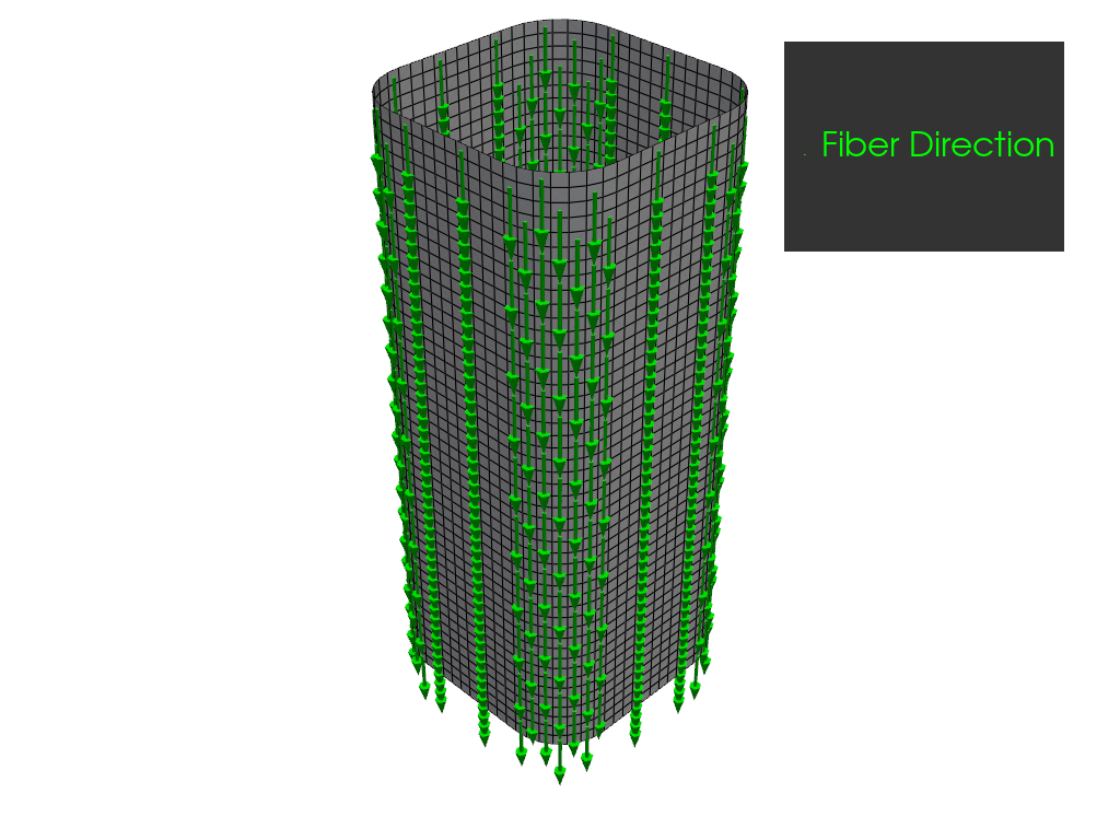
Create the ACP model and visualize the first ply’s fiber direction.
acp_workflow = prepare_acp_model(acp=acp_instance, workdir=workdir, input_file=input_file)
ply = list(acp_workflow.model.modeling_groups["Modeling_Group"].modeling_plies.values())[0]
pyacp.get_directions_plotter(
    model=acp_workflow.model,
    components=[ply.elemental_data.fiber_direction],
    length_factor=5.0,
    culling_factor=5,
).show()
Create functions for the optimization#
To optimize the ply angles, you must define functions to update, solve, and postprocess the ACP model for a given set of ply angles.
The update_ply_angles() function changes the ply angles in the model to the given values and
updates the model.
def update_ply_angles(*, acp_workflow, parameters):
    model = acp_workflow.model
    modeling_plies = list(model.modeling_groups["Modeling_Group"].modeling_plies.values())
    assert len(modeling_plies) == len(parameters)
    for angle, modeling_ply in zip(parameters, modeling_plies):
        modeling_ply.ply_angle = angle

    model.update()


update_ply_angles(acp_workflow=acp_workflow, parameters=[0, 45, 90, 135, 180, 225])
The solve_cdb() function solves the CDB file with MAPDL and returns the path to the RST file.
def solve_cdb(*, mapdl, cdb_file, workdir):
    mapdl.clear()
    mapdl.input(cdb_file)
    # Solve the model. Note that the model contains two timesteps.
    mapdl.allsel()
    mapdl.slashsolu()
    mapdl.time(1.0)
    mapdl.solve()
    mapdl.time(2.0)
    mapdl.solve()

    # Download the RST file for further postprocessing
    rstfile_name = f"{mapdl.jobname}.rst"
    rst_file_local_path = workdir / rstfile_name
    mapdl.download(rstfile_name, str(workdir))
    return rst_file_local_path


cdb_file = acp_workflow.get_local_cdb_file()
rst_file = solve_cdb(mapdl=mapdl, cdb_file=cdb_file, workdir=workdir)
The get_max_irf() function uses PyDPF Composites to calculate the maximum
inverse reserve factor (IRF) for a given RST, composite definitions,
or materials file.
This function only considers the maximum stress failure criterion.
max_stress_criterion = pydpf_composites.failure_criteria.MaxStressCriterion()
combined_failure_criterion = pydpf_composites.failure_criteria.CombinedFailureCriterion(
    name="Combined Failure Criterion",
    failure_criteria=[max_stress_criterion],
)


def get_max_irf(
    *,
    acp_workflow,
    dpf_server,
    rst_file,
    failure_criterion,
):
    # Create the composite model and configure its input
    composite_model = pydpf_composites.composite_model.CompositeModel(
        composite_files=pyacp.get_composite_post_processing_files(
            acp_workflow=acp_workflow,
            local_rst_file_path=rst_file,
        ),
        server=dpf_server,
    )

    def get_max_irf_for_time(time):
        """Compute the maximum IRF for a given time step."""
        output_all_elements = composite_model.evaluate_failure_criteria(
            failure_criterion,
            composite_scope=pydpf_composites.composite_scope.CompositeScope(time=time),
        )
        irf_field = output_all_elements.get_field(
            {"failure_label": pydpf_composites.constants.FailureOutput.FAILURE_VALUE}
        )
        return irf_field.max().data[0]

    return max(
        get_max_irf_for_time(time) for time in composite_model.get_result_times_or_frequencies()
    )


get_max_irf(
    acp_workflow=acp_workflow,
    dpf_server=dpf_server,
    rst_file=rst_file,
    failure_criterion=combined_failure_criterion,
)
1.402323456
Optimize the ply angles#
For the optimization, you must define a single function that takes the ply angles
as its input and returns the maximum IRF.
The get_max_irf_for_parameters() function combines the previously defined functions
to perform all the necessary steps for a given set of ply angles.
def get_max_irf_for_parameters(
    parameters, *, acp_workflow, mapdl, dpf_server, failure_criterion, workdir, results
):
    update_ply_angles(acp_workflow=acp_workflow, parameters=parameters)
    cdb_file = acp_workflow.get_local_cdb_file()
    rst_file = solve_cdb(mapdl=mapdl, cdb_file=cdb_file, workdir=workdir)
    res = get_max_irf(
        acp_workflow=acp_workflow,
        dpf_server=dpf_server,
        rst_file=rst_file,
        failure_criterion=failure_criterion,
    )
    results.append(res)
    print(f"Parameters: {parameters}, Max IRF: {res}")
    return res
To inject the acp_workflow, mapdl, dpf_server, and workdir arguments into the
get_max_irf_for_parameters() function, you can use the functools.partial() function.
results: list[float] = []
optimization_function = partial(
    get_max_irf_for_parameters,
    acp_workflow=acp_workflow,
    mapdl=mapdl,
    dpf_server=dpf_server,
    failure_criterion=combined_failure_criterion,
    workdir=workdir,
    results=results,
)
optimization_function([0, 45, 90, 135, 180, 225])
Parameters: [0, 45, 90, 135, 180, 225], Max IRF: 1.402323456

1.402323456
For the optimization, you can use the Nelder-Mead method available in
the scipy.optimize.minimize() function. This is a downhill simplex algorithm that
does not require the gradient of the objective function. It is suitable for finding
a local minimum of the objective function.
To have the Nelder-Mead method cover a reasonable part of the parameter space, define an initial simplex (matrix of shape (n+1, n), where n is the number of parameters).
The initial simplex is chosen with random ply angles between 0 and 90 degrees. To make the results reproducible, the random seed is fixed.
random.seed(42)
initial_simplex = [[random.uniform(0, 90) for _ in range(6)] for _ in range(7)]
To build this example, the number of function evaluations is limited to 1. In practice, you should increase or remove this limit.
maxfev = 1
res = minimize(
    optimization_function,
    [0, 0, 0, 0, 0, 0],
    method="Nelder-Mead",
    options={
        "disp": True,
        "initial_simplex": initial_simplex,
        "xatol": 1.0,
        "fatol": 0.001,
        "maxfev": maxfev,
    },
)
Parameters: [57.54841186 2.25096797 24.75263865 20.08896643 66.28240927 60.90295387], Max IRF: 1.251633536
Results#
Without the maxfev limit, the optimization would take roughly 30 minutes to complete and
converge to the following result:
>>> print(res)
       message: Optimization terminated successfully.
       success: True
        status: 0
           fun: 0.9129640864440078
             x: [ 7.826e+01  1.777e+00  1.042e+02  8.848e+01  1.083e+01
                 -1.288e+01]
           nit: 88
          nfev: 156
 final_simplex: (array([[ 7.826e+01,  1.777e+00, ...,  1.083e+01,
                        -1.288e+01],
                       [ 7.820e+01,  1.691e+00, ...,  1.046e+01,
                        -1.292e+01],
                       ...,
                       [ 7.821e+01,  1.067e+00, ...,  1.113e+01,
                        -1.299e+01],
                       [ 7.832e+01,  1.725e+00, ...,  1.090e+01,
                        -1.303e+01]]), array([ 9.130e-01,  9.130e-01,  9.132e-01,  9.133e-01,
                        9.133e-01,  9.133e-01,  9.134e-01]))
The following code defines the results list as it would be obtained from the full optimization.
# fmt: off
results = [
    1.251633536, 1.406139904, 1.400375936, 1.188398336, 1.292364032, 1.478680192,
    1.328360704, 1.403241856, 1.294695808, 1.499538048, 1.33415104, 1.34713472,
    1.313087872, 1.331134976, 1.3513568, 1.470391296, 1.42062272, 1.322532224,
    1.31974336, 1.373317248, 1.422083072, 1.343358464, 1.311241344, 1.316675968,
    1.340961792, 1.360485888, 1.343539456, 1.32766528, 1.270421504, 1.36705344,
    1.379165312, 1.322511232, 1.314317184, 1.223874304, 1.153106048, 1.007141504,
    1.05296512, 0.974143168, 0.9371091866404715, 0.9365409823182711, 0.9408823575638506,
    0.93918688, 0.994062912, 1.191067648, 0.9764623339882121, 0.938809398821218,
    0.9395024597249508, 0.99409632, 0.9367536031434185, 1.069221952, 0.9537923772102161,
    0.935515347740668, 1.069221952, 0.9373682043222004, 1.016040256, 0.9331018939096267,
    0.9388053752455796, 0.9323877092337918, 0.940058278978389, 0.9336497917485265,
    0.9311696345776032, 0.9494098231827112, 0.94191456, 0.9330088487229863, 0.9291408722986247,
    0.9445788290766208, 0.9506338703339882, 0.9252197721021611, 0.9309677013752455,
    0.929678648330059, 0.9256490373280943, 0.9378641100196463, 0.9268323457760315,
    0.9353581768172888, 0.9265237878192535, 0.9242050766208252, 0.9274993163064833,
    0.924646601178782, 0.9242514106090374, 0.9307412495088409, 0.9244120392927309,
    0.9209625776031434, 0.941085184, 0.9286979017681729, 0.9229924086444008,
    0.9197949233791749, 0.9203867033398822, 0.9217532730844794, 0.9229551905697446,
    0.9304816660117878, 0.9210226168958743, 0.9171427583497053, 0.929186496,
    0.9245868133595285, 0.9192841807465619, 0.9226500275049115, 0.9204163772102161,
    0.935395072, 0.9199762986247544, 0.9174358506876228, 0.9207507740667976,
    0.9191862946954813, 0.9187897838899803, 0.9173438742632612, 0.9179240235756385,
    0.916406208, 0.931066368, 0.93102176, 0.9173784518664048, 0.921966848,
    0.9165387819253438, 0.9182679764243615, 0.9152844950884086, 0.917331489194499,
    0.92203392, 0.9167768015717093, 0.9151537917485265, 0.9157055874263261,
    0.9171648251473478, 0.9157296031434184, 0.9149538703339882, 0.9153821925343811,
    0.9155963222003929, 0.9145536502946955, 0.916151232, 0.9177973438113949,
    0.9146214223968566, 0.9138568801571709, 0.913027206286837, 0.9152614223968566,
    0.9132077642436149, 0.9149754970530452, 0.917136512, 0.914141862475442,
    0.914945068762279, 0.914854978388998, 0.914139536345776, 0.9152915992141454,
    0.91376678978389, 0.9139345225933202, 0.9140565500982318, 0.9139955677799607,
    0.9152624911591356, 0.9134742632612967, 0.914016704, 0.9133683929273084,
    0.9141857445972495, 0.913588557956778, 0.9134601178781925, 0.9132596935166994,
    0.9138769351669941, 0.9133084793713163, 0.9129640864440078, 0.9130440550098232,
    0.9138289666011787, 0.9132928251473478
 ]
# fmt: on
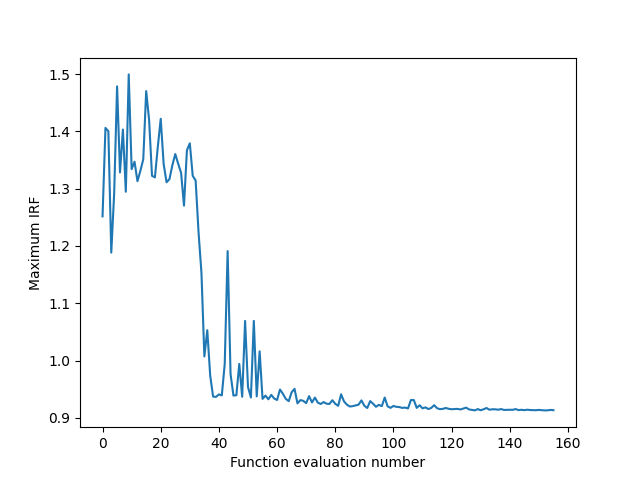
Visualize the evolution of the maximum IRF during the optimization.
fig, ax = plt.subplots()
ax.plot(results)
ax.set_xlabel("Function evaluation number")
ax.set_ylabel("Maximum IRF")
plt.show()
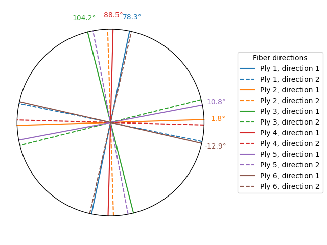
Visualize the resulting fiber directions.
angles_degree = [7.826e01, 1.777e00, 1.042e02, 8.848e01, 1.083e01, -1.288e01]

fig, ax = plt.subplots()
fig.subplots_adjust(right=0.65)

circle = patches.Circle((0, 0), radius=1, edgecolor="black", facecolor="none", zorder=10)
ax.add_patch(circle)

for i, angle_deg in enumerate(angles_degree):
    angle_rad = np.deg2rad(angle_deg)
    x = np.cos(angle_rad)
    y = np.sin(angle_rad)
    ax.plot(
        [-x, x],
        [-y, y],
        color=f"C{i}",
        label=f"Ply {i + 1}, direction 1",
    )
    # plot also the orthogonal direction, since the ply material is woven
    angle_ortho = angle_rad + np.pi / 2.0
    x_ortho = np.cos(angle_ortho)
    y_ortho = np.sin(angle_ortho)
    ax.plot(
        [-x_ortho, x_ortho],
        [-y_ortho, y_ortho],
        color=f"C{i}",
        linestyle="--",
        label=f"Ply {i + 1}, direction 2",
    )

    ax.text(x * 1.15, y * 1.15, f"{angle_deg:.1f}°", ha="center", va="center", color=f"C{i}")

ax.set_aspect("equal")
ax.legend(title="Fiber directions", loc="center left", bbox_to_anchor=(1.1, 0.5))

ax.axis("off")  # Hide the x and y axes

plt.tight_layout()
plt.show()
Total running time of the script: (0 minutes 48.270 seconds)