Note
Go to the end to download the full example code.
PyMAPDL workflow#
This example shows how to define a composite lay-up with PyACP, solve the resulting model with PyMAPDL, and run a failure analysis with PyDPF - Composites.
Description#
In a basic PyACP workflow, you begin with an MAPDL DAT file containing the mesh, material data, and
boundary conditions. For more information on creating input files, see Create input file for PyACP.
Then, you import the DAT file into PyACP to define the composite lay-up. Finally, you export the
resulting model from PyACP to PyMAPDL. Once the results are available, the RST file is loaded in
PyDPF - Composites for analysis. The additional input files (material.xml and
ACPCompositeDefinitions.h5) can also be stored with PyACP and passed to PyDPF - Composites.
Import modules#
Import the standard library and third-party dependencies.
import pathlib
import tempfile
Import the PyACP dependencies.
from ansys.acp.core import (
    PlyType,
    dpf_integration_helpers,
    get_directions_plotter,
    launch_acp,
    material_property_sets,
    print_model,
)
from ansys.acp.core.extras import ExampleKeys, get_example_file, set_plot_theme
Set the plot theme for the example. This is optional, and ensures that you get the same plot style (theme, color map, etc.) as in the online documentation.
set_plot_theme()
Launch PyACP#
Download the example input file.
tempdir = tempfile.TemporaryDirectory()
WORKING_DIR = pathlib.Path(tempdir.name)
input_file = get_example_file(ExampleKeys.BASIC_FLAT_PLATE_DAT, WORKING_DIR)
Launch the PyACP server and connect to it.
acp = launch_acp()
Import the model#
Import the model from the input DAT file.
model = acp.import_model(input_file, format="ansys:dat")
print(model.unit_system)
mks
Visualize the loaded mesh.
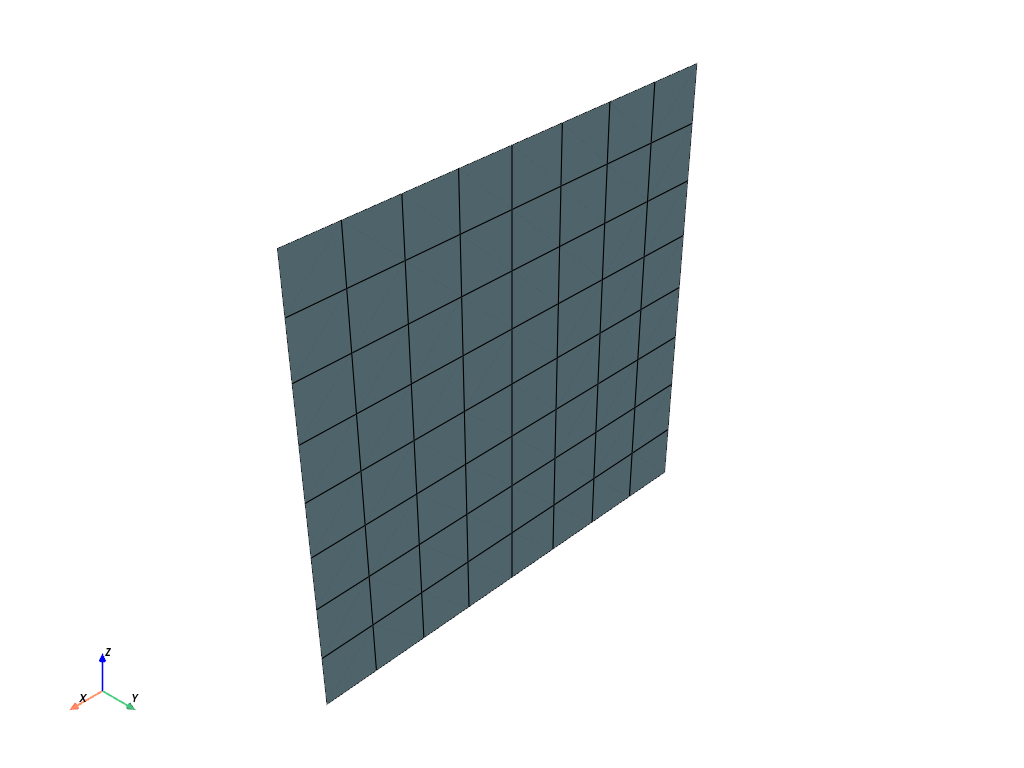
Define the composite lay-up#
Create an orthotropic material and fabric including strain limits, which are later used to postprocess the simulation.
engineering_constants = (
    material_property_sets.ConstantEngineeringConstants.from_orthotropic_constants(
        E1=5e10, E2=1e10, E3=1e10, nu12=0.28, nu13=0.28, nu23=0.3, G12=5e9, G23=4e9, G31=4e9
    )
)

strain_limit = 0.01
strain_limits = material_property_sets.ConstantStrainLimits.from_orthotropic_constants(
    eXc=-strain_limit,
    eYc=-strain_limit,
    eZc=-strain_limit,
    eXt=strain_limit,
    eYt=strain_limit,
    eZt=strain_limit,
    eSxy=strain_limit,
    eSyz=strain_limit,
    eSxz=strain_limit,
)

ud_material = model.create_material(
    name="UD",
    ply_type=PlyType.REGULAR,
    engineering_constants=engineering_constants,
    strain_limits=strain_limits,
)

fabric = model.create_fabric(name="UD", material=ud_material, thickness=0.1)
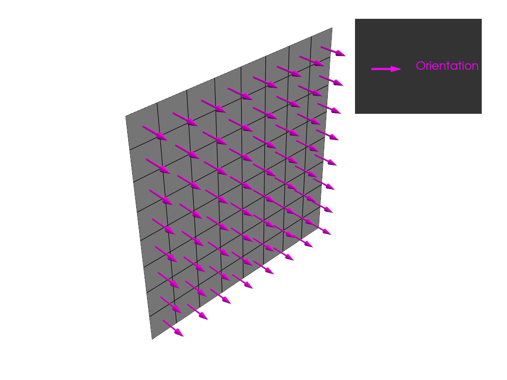
Define a rosette and oriented selection set. Plot the orientation.
rosette = model.create_rosette(origin=(0.0, 0.0, 0.0), dir1=(1.0, 0.0, 0.0), dir2=(0.0, 0.0, 1.0))

oss = model.create_oriented_selection_set(
    name="oss",
    orientation_point=(0.0, 0.0, 0.0),
    orientation_direction=(0.0, 1.0, 0),
    element_sets=[model.element_sets["All_Elements"]],
    rosettes=[rosette],
)

model.update()

plotter = get_directions_plotter(model=model, components=[oss.elemental_data.orientation])
plotter.show()
Create various plies with different angles and add them to a modeling group.
modeling_group = model.create_modeling_group(name="modeling_group")
angles = [0, 45, -45, 45, -45, 0]
for idx, angle in enumerate(angles):
    modeling_group.create_modeling_ply(
        name=f"ply_{idx}_{angle}_{fabric.name}",
        ply_angle=angle,
        ply_material=fabric,
        oriented_selection_sets=[oss],
    )

model.update()
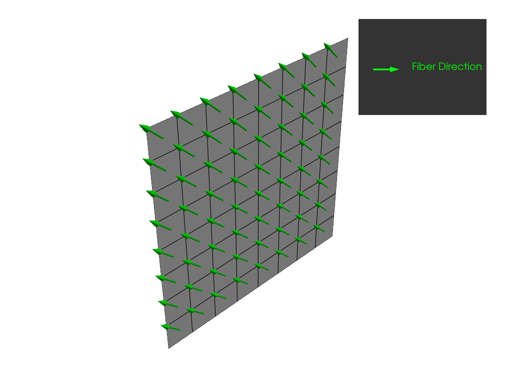
Show the fiber directions of a specific ply.
modeling_ply = model.modeling_groups["modeling_group"].modeling_plies["ply_4_-45_UD"]


fiber_direction = modeling_ply.elemental_data.fiber_direction
assert fiber_direction is not None
plotter = get_directions_plotter(
    model=model,
    components=[fiber_direction],
)

plotter.show()
For a quick overview, print the model tree. Note that the model can also be opened in the ACP GUI. For more information, see View model in ACP GUI.
print_model(model)
'ACP Lay-up Model'
    Materials
        '1'
        'UD'
    Fabrics
        'UD'
    Element Sets
        'All_Elements'
    Edge Sets
        '_FIXEDSU'
    Rosettes
        '12'
        'Rosette'
    Oriented Selection Sets
        'oss'
    Modeling Groups
        'modeling_group'
            Modeling Plies
                'ply_0_0_UD'
                    Production Plies
                        'P1__ply_0_0_UD'
                            Analysis Plies
                                'P1L1__ply_0_0_UD'
                'ply_1_45_UD'
                    Production Plies
                        'P1__ply_1_45_UD'
                            Analysis Plies
                                'P1L1__ply_1_45_UD'
                'ply_2_-45_UD'
                    Production Plies
                        'P1__ply_2_-45_UD'
                            Analysis Plies
                                'P1L1__ply_2_-45_UD'
                'ply_3_45_UD'
                    Production Plies
                        'P1__ply_3_45_UD'
                            Analysis Plies
                                'P1L1__ply_3_45_UD'
                'ply_4_-45_UD'
                    Production Plies
                        'P1__ply_4_-45_UD'
                            Analysis Plies
                                'P1L1__ply_4_-45_UD'
                'ply_5_0_UD'
                    Production Plies
                        'P1__ply_5_0_UD'
                            Analysis Plies
                                'P1L1__ply_5_0_UD'
Solve the model with PyMAPDL#
Launch the PyMAPDL instance.
from ansys.mapdl.core import launch_mapdl

mapdl = launch_mapdl()
mapdl.clear()
/home/runner/work/pyacp/pyacp/.venv/lib/python3.14/site-packages/ansys/tools/common/cyberchannel.py:201: UserWarning: Starting gRPC client without TLS on 127.0.0.1:50557. This is INSECURE. Consider using a secure connection.
  warn(f"Starting gRPC client without TLS on {target}. This is INSECURE. Consider using a secure connection.")
Load the CDB file into PyMAPDL.
analysis_model_path = WORKING_DIR / "analysis_model.cdb"
model.export_analysis_model(analysis_model_path)
mapdl.input(str(analysis_model_path))
'\n /INPUT FILE= LINE= 0\n\n\n\n DO NOT WRITE ELEMENT RESULTS INTO DATABASE\n\n *GET _WALLSTRT FROM ACTI ITEM=TIME WALL VALUE= 0.772627738E-01\n\n TITLE= \n wbnew--Static Structural (A5) \n\n ACT Extensions:\n LSDYNA, 2024.1\n 5f463412-bd3e-484b-87e7-cbc0a665e474, wbex\n /COM, ANSYSMotion, 2024.2\n 20180725-3f81-49eb-9f31-41364844c769, wbex\n \n\n SET PARAMETER DIMENSIONS ON _WB_PROJECTSCRATCH_DIR\n TYPE=STRI DIMENSIONS= 248 1 1\n\n PARAMETER _WB_PROJECTSCRATCH_DIR(1) = D:\\ARM_Reports\\ACP_IMP_LAY_SEC_037_01102024082855\\TBSolves\\WB_jvonrick_50936_2\\wbnew_files\\dp0\\SYS\\MECH\\\n\n SET PARAMETER DIMENSIONS ON _WB_SOLVERFILES_DIR\n TYPE=STRI DIMENSIONS= 248 1 1\n\n PARAMETER _WB_SOLVERFILES_DIR(1) = D:\\ARM_Reports\\ACP_IMP_LAY_SEC_037_01102024082855\\TBSolves\\WB_jvonrick_50936_2\\wbnew_files\\dp0\\SYS\\MECH\\\n\n SET PARAMETER DIMENSIONS ON _WB_USERFILES_DIR\n TYPE=STRI DIMENSIONS= 248 1 1\n\n PARAMETER _WB_USERFILES_DIR(1) = D:\\ARM_Reports\\ACP_IMP_LAY_SEC_037_01102024082855\\TBSolves\\WB_jvonrick_50936_2\\wbnew_files\\user_files\\\n --- Data in consistent MKS units. See Solving Units in the help system for more\n\n MKS UNITS SPECIFIED FOR INTERNAL \n LENGTH (l) = METER (M)\n MASS (M) = KILOGRAM (KG)\n TIME (t) = SECOND (SEC)\n TEMPERATURE (T) = CELSIUS (C)\n TOFFSET = 273.0\n CHARGE (Q) = COULOMB\n FORCE (f) = NEWTON (N) (KG-M/SEC2)\n HEAT = JOULE (N-M)\n\n PRESSURE = PASCAL (NEWTON/M**2)\n ENERGY (W) = JOULE (N-M)\n POWER (P) = WATT (N-M/SEC)\n CURRENT (i) = AMPERE (COULOMBS/SEC)\n CAPACITANCE (C) = FARAD\n INDUCTANCE (L) = HENRY\n MAGNETIC FLUX = WEBER\n RESISTANCE (R) = OHM\n ELECTRIC POTENTIAL = VOLT\n\n INPUT UNITS ARE ALSO SET TO MKS \n *****MAPDL VERIFICATION RUN ONLY*****\n DO NOT USE RESULTS FOR PRODUCTION\n\n ***** MAPDL ANALYSIS DEFINITION (PREP7) *****\n *********** Nodes for the whole assembly ***********\n *********** Elements for Body 1 "SYS\\Surface" ***********\n *********** Send User Defined Coordinate System(s) ***********\n *********** Set Reference Temperature ***********\n *********** Send Materials ***********\n *********** Send Sheet Properties ***********\n *********** Fixed Supports ***********\n *********** Define Force Using Surface Effect Elements ***********\n\n\n ***** ROUTINE COMPLETED ***** ELAPSED TIME = 0.000\n\n\n --- Number of total nodes = 81\n --- Number of contact elements = 8\n --- Number of spring elements = 0\n --- Number of bearing elements = 0\n --- Number of solid elements = 64\n --- Number of condensed parts = 0\n --- Number of total elements = 72\n\n *GET _WALLBSOL FROM ACTI ITEM=TIME WALL VALUE= 0.772635048E-01\n ****************************************************************************\n ************************* SOLUTION ********************************\n ****************************************************************************\n\n ***** MAPDL SOLUTION ROUTINE *****\n\n\n PERFORM A STATIC ANALYSIS\n THIS WILL BE A NEW ANALYSIS\n\n PARAMETER _THICKRATIO = 0.000000000 \n\n USE SPARSE MATRIX DIRECT SOLVER\n\n CONTACT INFORMATION PRINTOUT LEVEL 1\n\n CHECK INITIAL OPEN/CLOSED STATUS OF SELECTED CONTACT ELEMENTS\n AND LIST DETAILED CONTACT PAIR INFORMATION\n\n SPLIT CONTACT SURFACES AT SOLVE PHASE\n\n NUMBER OF SPLITTING TBD BY PROGRAM\n\n DO NOT COMBINE ELEMENT MATRIX FILES (.emat) AFTER DISTRIBUTED PARALLEL SOLUTION\n\n DO NOT COMBINE ELEMENT SAVE DATA FILES (.esav) AFTER DISTRIBUTED PARALLEL SOLUTION\n\n NLDIAG: Nonlinear diagnostics CONT option is set to ON. \n Writing frequency : each ITERATION.\n\n DO NOT SAVE ANY RESTART FILES AT ALL\n ****************************************************\n ******************* SOLVE FOR LS 1 OF 1 ****************\n\n SELECT FOR ITEM=TYPE COMPONENT= \n IN RANGE 2 TO 2 STEP 1\n\n 8 ELEMENTS (OF 72 DEFINED) SELECTED BY ESEL COMMAND.\n\n SELECT ALL NODES HAVING ANY ELEMENT IN ELEMENT SET.\n\n 9 NODES (OF 81 DEFINED) SELECTED FROM\n 8 SELECTED ELEMENTS BY NSLE COMMAND.\n\n SPECIFIED SURFACE LOAD PRES FOR ALL SELECTED ELEMENTS LKEY = 1 KVAL = 1\n VALUES = 0.0000 0.0000 0.0000 0.0000 \n\n SPECIFIED SURFACE LOAD PRES FOR ALL SELECTED ELEMENTS LKEY = 2 KVAL = 1\n VALUES = -10000. -10000. -10000. -10000. \n\n SPECIFIED SURFACE LOAD PRES FOR ALL SELECTED ELEMENTS LKEY = 3 KVAL = 1\n VALUES = 0.0000 0.0000 0.0000 0.0000 \n\n ALL SELECT FOR ITEM=NODE COMPONENT= \n IN RANGE 1 TO 81 STEP 1\n\n 81 NODES (OF 81 DEFINED) SELECTED BY NSEL COMMAND.\n\n ALL SELECT FOR ITEM=ELEM COMPONENT= \n IN RANGE 1 TO 72 STEP 1\n\n 72 ELEMENTS (OF 72 DEFINED) SELECTED BY ESEL COMMAND.\n\n PRINTOUT RESUMED BY /GOP\n\n USE 1 SUBSTEPS INITIALLY THIS LOAD STEP FOR ALL DEGREES OF FREEDOM\n FOR AUTOMATIC TIME STEPPING:\n USE 1 SUBSTEPS AS A MAXIMUM\n USE 1 SUBSTEPS AS A MINIMUM\n\n TIME= 1.0000 \n\n ERASE THE CURRENT DATABASE OUTPUT CONTROL TABLE.\n\n\n WRITE ALL ITEMS TO THE DATABASE WITH A FREQUENCY OF NONE\n FOR ALL APPLICABLE ENTITIES\n\n WRITE NSOL ITEMS TO THE DATABASE WITH A FREQUENCY OF ALL \n FOR ALL APPLICABLE ENTITIES\n\n WRITE RSOL ITEMS TO THE DATABASE WITH A FREQUENCY OF ALL \n FOR ALL APPLICABLE ENTITIES\n\n WRITE EANG ITEMS TO THE DATABASE WITH A FREQUENCY OF ALL \n FOR ALL APPLICABLE ENTITIES\n\n WRITE ETMP ITEMS TO THE DATABASE WITH A FREQUENCY OF ALL \n FOR ALL APPLICABLE ENTITIES\n\n WRITE VENG ITEMS TO THE DATABASE WITH A FREQUENCY OF ALL \n FOR ALL APPLICABLE ENTITIES\n\n WRITE STRS ITEMS TO THE DATABASE WITH A FREQUENCY OF ALL \n FOR ALL APPLICABLE ENTITIES\n\n WRITE EPEL ITEMS TO THE DATABASE WITH A FREQUENCY OF ALL \n FOR ALL APPLICABLE ENTITIES\n\n WRITE EPPL ITEMS TO THE DATABASE WITH A FREQUENCY OF ALL \n FOR ALL APPLICABLE ENTITIES\n\n WRITE CONT ITEMS TO THE DATABASE WITH A FREQUENCY OF ALL \n FOR ALL APPLICABLE ENTITIES\n\n *GET ANSINTER_ FROM ACTI ITEM=INT VALUE= 0.00000000 \n\n *IF ANSINTER_ ( = 0.00000 ) NE \n 0 ( = 0.00000 ) THEN \n\n *ENDIF\n\n ***** MAPDL SOLVE COMMAND *****\n\n *** WARNING *** ELAPSED TIME = 0.000 TIME= 00:00:00\n Element shape checking is currently inactive. Issue SHPP,ON or \n SHPP,WARN to reactivate, if desired. \n\n *** NOTE *** ELAPSED TIME = 0.000 TIME= 00:00:00\n The model data was checked and warning messages were found. \n Please review output or errors file ( ) for these warning messages. \n *****MAPDL VERIFICATION RUN ONLY*****\n DO NOT USE RESULTS FOR PRODUCTION\n\n S O L U T I O N O P T I O N S\n\n PROBLEM DIMENSIONALITY. . . . . . . . . . . . .3-D \n DEGREES OF FREEDOM. . . . . . UX UY UZ ROTX ROTY ROTZ\n ANALYSIS TYPE . . . . . . . . . . . . . . . . .STATIC (STEADY-STATE)\n OFFSET TEMPERATURE FROM ABSOLUTE ZERO . . . . . 273.15 \n EQUATION SOLVER OPTION. . . . . . . . . . . . .SPARSE \n GLOBALLY ASSEMBLED MATRIX . . . . . . . . . . .SYMMETRIC \n\n *** NOTE *** ELAPSED TIME = 0.000 TIME= 00:00:00\n Poisson\'s ratio PR input has been converted to NU input. \n\n L O A D S T E P O P T I O N S\n\n LOAD STEP NUMBER. . . . . . . . . . . . . . . . 1\n TIME AT END OF THE LOAD STEP. . . . . . . . . . 1.0000 \n NUMBER OF SUBSTEPS. . . . . . . . . . . . . . . 1\n STEP CHANGE BOUNDARY CONDITIONS . . . . . . . . NO\n PRINT OUTPUT CONTROLS . . . . . . . . . . . . .NO PRINTOUT\n DATABASE OUTPUT CONTROLS\n ITEM FREQUENCY COMPONENT\n ALL NONE \n NSOL ALL \n RSOL ALL \n EANG ALL \n ETMP ALL \n VENG ALL \n STRS ALL \n EPEL ALL \n EPPL ALL \n CONT ALL \n\n\n *** NOTE *** ELAPSED TIME = 0.000 TIME= 00:00:00\n Predictor is ON by default for structural elements with rotational \n degrees of freedom. Use the PRED,OFF command to turn the predictor \n OFF if it adversely affects the convergence. \n\n\n Range of element maximum matrix coefficients in global coordinates\n Maximum = 8.014568245E+11 at element 0. \n Minimum = 8.014568181E+11 at element 0. \n\n *** ELEMENT MATRIX FORMULATION TIMES\n TYPE NUMBER ENAME TOTAL ELAPSED AVG ELAPSED\n\n 1 64 SHELL181 0.0000 0.000000000\n 2 8 SURF156 0.0000 0.000000000\n Elapsed Time at end of element matrix formulation = 0. \n\n SPARSE MATRIX DIRECT SOLVER.\n Number of equations = 432, Maximum wavefront = 0\n Memory available (MB) = 0.0 , Memory required (MB) = 0.0 \n\n Sparse solver maximum pivot= 0 at node 0 . \n Sparse solver minimum pivot= 0 at node 0 . \n Sparse solver minimum pivot in absolute value= 0 at node 0 . \n\n *** ELEMENT RESULT CALCULATION TIMES\n TYPE NUMBER ENAME TOTAL ELAPSED AVG ELAPSED\n\n 1 64 SHELL181 0.0000 0.000000000\n 2 8 SURF156 0.0000 0.000000000\n\n *** NODAL LOAD CALCULATION TIMES\n TYPE NUMBER ENAME TOTAL ELAPSED AVG ELAPSED\n\n 1 64 SHELL181 0.0000 0.000000000\n 2 8 SURF156 0.0000 0.000000000\n *** LOAD STEP 1 SUBSTEP 1 COMPLETED. CUM ITER = 1\n *** TIME = 1.00000 TIME INC = 1.00000 NEW TRIANG MATRIX\n *************** Write FE CONNECTORS *********\n\n WRITE OUT CONSTRAINT EQUATIONS TO FILE= \n ****************************************************\n *************** FINISHED SOLVE FOR LS 1 *************\n\n *GET _WALLASOL FROM ACTI ITEM=TIME WALL VALUE= 0.772798643E-01\n\n PRINTOUT RESUMED BY /GOP\n\n FINISH SOLUTION PROCESSING\n\n\n ***** ROUTINE COMPLETED ***** ELAPSED TIME = 0.000\n\n\n *****MAPDL VERIFICATION RUN ONLY*****\n DO NOT USE RESULTS FOR PRODUCTION\n\n ***** MAPDL RESULTS INTERPRETATION (POST1) *****\n\n Set Encoding of XML File to:ISO-8859-1\n\n Set Output of XML File to:\n PARM, , , , , , , , , , , ,\n , , , , , , ,\n\n DATABASE WRITTEN ON FILE parm.xml \n\n EXIT THE MAPDL POST1 DATABASE PROCESSOR\n\n\n ***** ROUTINE COMPLETED ***** ELAPSED TIME = 0.000\n\n\n\n PRINTOUT RESUMED BY /GOP\n\n *GET _WALLDONE FROM ACTI ITEM=TIME WALL VALUE= 0.772803725E-01\n\n PARAMETER _PREPTIME = 0.2631685842E-02\n\n PARAMETER _SOLVTIME = 0.5889435129E-01\n\n PARAMETER _POSTTIME = 0.1829403509E-02\n\n PARAMETER _TOTALTIM = 0.6335544064E-01\n\n *GET _DLBRATIO FROM ACTI ITEM=SOLU DLBR VALUE= 0.00000000 \n\n *GET _COMBTIME FROM ACTI ITEM=SOLU COMB VALUE= 0.00000000 \n\n *GET _SSMODE FROM ACTI ITEM=SOLU SSMM VALUE= 2.00000000 \n\n *GET _NDOFS FROM ACTI ITEM=SOLU NDOF VALUE= 432.000000 \n\n *GET _SOL_END_TIME FROM ACTI ITEM=SET TIME VALUE= 1.00000000 \n\n *IF _sol_end_time ( = 1.00000 ) EQ \n 1.000000 ( = 1.00000 ) THEN \n\n /FCLEAN COMMAND REMOVING ALL LOCAL FILES\n\n *ENDIF\n --- Total number of nodes = 81\n --- Total number of elements = 72\n --- Element load balance ratio = 0\n --- Time to combine distributed files = 0\n --- Sparse memory mode = 2\n --- Number of DOF = 432\n'
Solve the model.
mapdl.allsel()
mapdl.slashsolu()
mapdl.solve()
*****  MAPDL SOLVE    COMMAND  *****

 *** WARNING ***                         ELAPSED TIME =       0.000   TIME= 00:00:00
 Element shape checking is currently inactive.  Issue SHPP,ON or
 SHPP,WARN to reactivate, if desired.

 *** NOTE ***                            ELAPSED TIME =       0.000   TIME= 00:00:00
 The model data was checked and warning messages were found.
  Please review output or errors file ( ) for these warning messages.
   *****MAPDL VERIFICATION RUN ONLY*****
     DO NOT USE RESULTS FOR PRODUCTION

                       S O L U T I O N   O P T I O N S

   PROBLEM DIMENSIONALITY. . . . . . . . . . . . .3-D
   DEGREES OF FREEDOM. . . . . . UX   UY   UZ   ROTX ROTY ROTZ
   ANALYSIS TYPE . . . . . . . . . . . . . . . . .STATIC (STEADY-STATE)
   OFFSET TEMPERATURE FROM ABSOLUTE ZERO . . . . .  273.15
   EQUATION SOLVER OPTION. . . . . . . . . . . . .SPARSE
   GLOBALLY ASSEMBLED MATRIX . . . . . . . . . . .SYMMETRIC

                      L O A D   S T E P   O P T I O N S

   LOAD STEP NUMBER. . . . . . . . . . . . . . . .     1
   TIME AT END OF THE LOAD STEP. . . . . . . . . .  1.0000
   NUMBER OF SUBSTEPS. . . . . . . . . . . . . . .     1
   STEP CHANGE BOUNDARY CONDITIONS . . . . . . . .    NO
   PRINT OUTPUT CONTROLS . . . . . . . . . . . . .NO PRINTOUT
   DATABASE OUTPUT CONTROLS
      ITEM     FREQUENCY   COMPONENT
       ALL       NONE
      NSOL        ALL
      RSOL        ALL
      EANG        ALL
      ETMP        ALL
      VENG        ALL
      STRS        ALL
      EPEL        ALL
      EPPL        ALL
      CONT        ALL


 *** NOTE ***                            ELAPSED TIME =       0.000   TIME= 00:00:00
 Predictor is ON by default for structural elements with rotational
 degrees of freedom.  Use the PRED,OFF command to turn the predictor
 OFF if it adversely affects the convergence.


 Range of element maximum matrix coefficients in global coordinates
 Maximum = 8.014568245E+11 at element 0.
 Minimum = 8.014568181E+11 at element 0.

   *** ELEMENT MATRIX FORMULATION TIMES
     TYPE    NUMBER     ENAME   TOTAL ELAPSED   AVG ELAPSED

        1        64  SHELL181          0.0000   0.000000000
        2         8   SURF156          0.0000   0.000000000
 Elapsed Time at end of element matrix formulation = 0.

 SPARSE MATRIX DIRECT SOLVER.
  Number of equations =         432,    Maximum wavefront =      0
  Memory available (MB) =    0.0    ,  Memory required (MB) =    0.0

 Sparse solver maximum pivot= 0 at node 0 .
 Sparse solver minimum pivot= 0 at node 0 .
 Sparse solver minimum pivot in absolute value= 0 at node 0 .

   *** ELEMENT RESULT CALCULATION TIMES
     TYPE    NUMBER     ENAME   TOTAL ELAPSED   AVG ELAPSED

        1        64  SHELL181          0.0000   0.000000000
        2         8   SURF156          0.0000   0.000000000

   *** NODAL LOAD CALCULATION TIMES
     TYPE    NUMBER     ENAME   TOTAL ELAPSED   AVG ELAPSED

        1        64  SHELL181          0.0000   0.000000000
        2         8   SURF156          0.0000   0.000000000
 *** LOAD STEP     1   SUBSTEP     1  COMPLETED.    CUM ITER =      1
 *** TIME =   1.00000         TIME INC =   1.00000      NEW TRIANG MATRIX
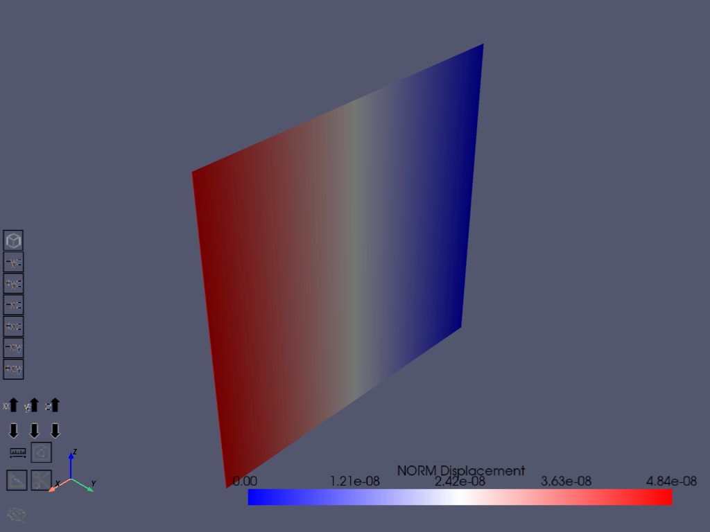
Show the displacements in postprocessing.
mapdl.post1()
mapdl.set("last")
mapdl.post_processing.plot_nodal_displacement(component="NORM")
/home/runner/work/pyacp/pyacp/.venv/lib/python3.14/site-packages/ansys/mapdl/core/mesh_grpc.py:103: PyVistaFutureWarning: The default value of `algorithm` for the filter
`UnstructuredGrid.extract_surface` will change in the future. It currently defaults to
`'dataset_surface'`, but will change to `None`. Explicitly set the `algorithm` keyword to
silence this warning.
  self._surf_cache = self._grid.extract_surface()
[84, 89, 109]
Download the RST file for composite-specific postprocessing.
rstfile_name = f"{mapdl.jobname}.rst"
rst_file_local_path = WORKING_DIR / rstfile_name
mapdl.download(rstfile_name, str(WORKING_DIR))
['file.rst']
Postprocessing with PyDPF - Composites#
To postprocess the results, you must configure the imports, connect to the PyDPF - Composites server, and load its plugin.
from ansys.dpf.composites.composite_model import CompositeModel
from ansys.dpf.composites.constants import FailureOutput
from ansys.dpf.composites.data_sources import (
    CompositeDefinitionFiles,
    ContinuousFiberCompositesFiles,
)
from ansys.dpf.composites.failure_criteria import CombinedFailureCriterion, MaxStrainCriterion
from ansys.dpf.composites.server_helpers import connect_to_or_start_server
Connect to the server. The connect_to_or_start_server function
automatically loads the composites plugin.
dpf_server = connect_to_or_start_server()
Specify the combined failure criterion.
max_strain = MaxStrainCriterion()

cfc = CombinedFailureCriterion(
    name="Combined Failure Criterion",
    failure_criteria=[max_strain],
)
Create the composite model and configure its input.
composite_definitions_file = WORKING_DIR / "ACPCompositeDefinitions.h5"
model.export_shell_composite_definitions(composite_definitions_file)
materials_file = WORKING_DIR / "materials.xml"
model.export_materials(materials_file)
composite_model = CompositeModel(
    composite_files=ContinuousFiberCompositesFiles(
        rst=rst_file_local_path,
        composite={"shell": CompositeDefinitionFiles(composite_definitions_file)},
        engineering_data=materials_file,
    ),
    default_unit_system=dpf_integration_helpers.get_dpf_unit_system(model.unit_system),
    server=dpf_server,
)
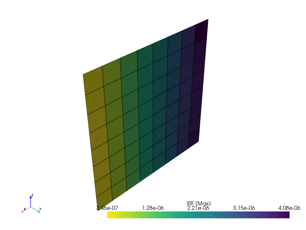
Evaluate and plot the failure criteria.
output_all_elements = composite_model.evaluate_failure_criteria(cfc)
irf_field = output_all_elements.get_field({"failure_label": FailureOutput.FAILURE_VALUE})
irf_field.plot()
(None, <pyvista.plotting.plotter.Plotter object at 0x7f7f7d3be850>)
Release the composite model to close the open streams to the result file.
composite_model = None  # type: ignore

# Close MAPDL instance
mapdl.exit()
Total running time of the script: (0 minutes 20.633 seconds)