Note
Go to the end to download the full example code.
Advanced PyMAPDL workflow#
This example shows how to define a composite lay-up with PyACP, solve the resulting model with PyMAPDL, and run a failure analysis with PyDPF - Composites.
Begin with an MAPDL CDB file that contains the mesh, material data, and
boundary conditions. Import the file to PyACP to define the lay-up, and then export the
resulting model to PyMAPDL. Once the results are available, the RST file is loaded in
PyDPF - Composites for postprocessing. The additional input files (material.xml
and ACPCompositeDefinitions.h5) can also be stored with PyACP and passed to PyDPF - Composites.
Import modules and start ACP#
Import the standard library and third-party dependencies.
import pathlib
import tempfile

import pyvista
Import the Ansys libraries.
import ansys.acp.core as pyacp
from ansys.acp.core.extras import set_plot_theme
Set the plot theme for the example. This is optional, and ensures that you get the same plot style (theme, color map, etc.) as in the online documentation.
set_plot_theme()
Launch the PyACP server and connect to it.
acp = pyacp.launch_acp()
Get example input files#
Create a temporary working directory, and download the example input files to this directory.
working_dir = tempfile.TemporaryDirectory()
working_dir_path = pathlib.Path(working_dir.name)
input_file = pyacp.extras.example_helpers.get_example_file(
    pyacp.extras.example_helpers.ExampleKeys.CLASS40_CDB, working_dir_path
)
Load mesh and materials from CDB file#
Load the CDB file into PyACP and set the unit system.
model = acp.import_model(path=input_file, format="ansys:cdb", unit_system=pyacp.UnitSystemType.MKS)
model
<Model with name 'ACP Lay-up Model'>
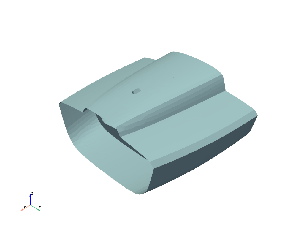
Visualize the loaded mesh.
Build Composite Lay-up#
Create the model (MKS unit system).
Materials#
mat_corecell_81kg = model.materials["1"]
mat_corecell_81kg.name = "Core Cell 81kg"
mat_corecell_81kg.ply_type = "isotropic_homogeneous_core"

mat_corecell_103kg = model.materials["2"]
mat_corecell_103kg.name = "Core Cell 103kg"
mat_corecell_103kg.ply_type = "isotropic_homogeneous_core"

mat_eglass_ud = model.materials["3"]
mat_eglass_ud.name = "E-Glass (uni-directional)"
mat_eglass_ud.ply_type = "regular"
Fabrics#
corecell_81kg_5mm = model.create_fabric(
    name="Corecell 81kg", thickness=0.005, material=mat_corecell_81kg
)
corecell_103kg_10mm = model.create_fabric(
    name="Corecell 103kg", thickness=0.01, material=mat_corecell_103kg
)
eglass_ud_02mm = model.create_fabric(name="eglass UD", thickness=0.0002, material=mat_eglass_ud)
Rosettes#
ros_deck = model.create_rosette(name="ros_deck", origin=(-5.9334, -0.0481, 1.693))
ros_hull = model.create_rosette(name="ros_hull", origin=(-5.3711, -0.0506, -0.2551))
ros_bulkhead = model.create_rosette(
    name="ros_bulkhead", origin=(-5.622, 0.0022, 0.0847), dir1=(0.0, 1.0, 0.0), dir2=(0.0, 0.0, 1.0)
)
ros_keeltower = model.create_rosette(
    name="ros_keeltower", origin=(-6.0699, -0.0502, 0.623), dir1=(0.0, 0.0, 1.0)
)
Oriented Selection Sets#
Note that the element sets are imported from the initial mesh (CBD file).
oss_deck = model.create_oriented_selection_set(
    name="oss_deck",
    orientation_point=(-5.3806, -0.0016, 1.6449),
    orientation_direction=(0.0, 0.0, -1.0),
    element_sets=[model.element_sets["DECK"]],
    rosettes=[ros_deck],
)

oss_hull = model.create_oriented_selection_set(
    name="oss_hull",
    orientation_point=(-5.12, 0.1949, -0.2487),
    orientation_direction=(0.0, 0.0, 1.0),
    element_sets=[model.element_sets["HULL_ALL"]],
    rosettes=[ros_hull],
)

oss_bulkhead = model.create_oriented_selection_set(
    name="oss_bulkhead",
    orientation_point=(-5.622, -0.0465, -0.094),
    orientation_direction=(1.0, 0.0, 0.0),
    element_sets=[model.element_sets["BULKHEAD_ALL"]],
    rosettes=[ros_bulkhead],
)

esets = [
    model.element_sets["KEELTOWER_AFT"],
    model.element_sets["KEELTOWER_FRONT"],
    model.element_sets["KEELTOWER_PORT"],
    model.element_sets["KEELTOWER_STB"],
]

oss_keeltower = model.create_oriented_selection_set(
    name="oss_keeltower",
    orientation_point=(-6.1019, 0.0001, 1.162),
    orientation_direction=(-1.0, 0.0, 0.0),
    element_sets=esets,
    rosettes=[ros_keeltower],
)
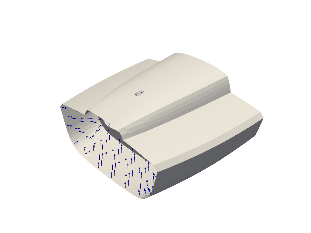
Show the orientations on the hull oriented selection set (OSS).
Note that the model must be updated before the orientations are available.
model.update()

plotter = pyvista.Plotter()
plotter.add_mesh(model.mesh.to_pyvista(), color="white")
orientation = oss_hull.elemental_data.orientation
assert orientation is not None
plotter.add_mesh(
    orientation.get_pyvista_glyphs(mesh=model.mesh, factor=0.2, culling_factor=5),
    color="blue",
)
plotter.show()
Modeling Plies#
Define plies for the hull, deck, and bulkhead.
angles = [-90.0, -60.0, -45.0 - 30.0, 0.0, 0.0, 30.0, 45.0, 60.0, 90.0]
for mg_name in ["hull", "deck", "bulkhead"]:
    mg = model.create_modeling_group(name=mg_name)
    oss_list = [model.oriented_selection_sets["oss_" + mg_name]]
    for angle in angles:
        add_ply(mg, "eglass_ud_02mm_" + str(angle), eglass_ud_02mm, angle, oss_list)
    add_ply(mg, "corecell_103kg_10mm", corecell_103kg_10mm, 0.0, oss_list)
    for angle in angles:
        add_ply(mg, "eglass_ud_02mm_" + str(angle), eglass_ud_02mm, angle, oss_list)
Add plies to the keeltower.
mg = model.create_modeling_group(name="keeltower")
oss_list = [model.oriented_selection_sets["oss_keeltower"]]
for angle in angles:
    add_ply(mg, "eglass_ud_02mm_" + str(angle), eglass_ud_02mm, angle, oss_list)

add_ply(mg, "corecell_81kg_5mm", corecell_81kg_5mm, 0.0, oss_list)

for angle in angles:
    add_ply(mg, "eglass_ud_02mm_" + str(angle), eglass_ud_02mm, angle, oss_list)
Inspect the number of modeling groups and plies.
print(len(model.modeling_groups))
print(len(model.modeling_groups["hull"].modeling_plies))
print(len(model.modeling_groups["deck"].modeling_plies))
print(len(model.modeling_groups["bulkhead"].modeling_plies))
print(len(model.modeling_groups["keeltower"].modeling_plies))
4
19
19
19
19
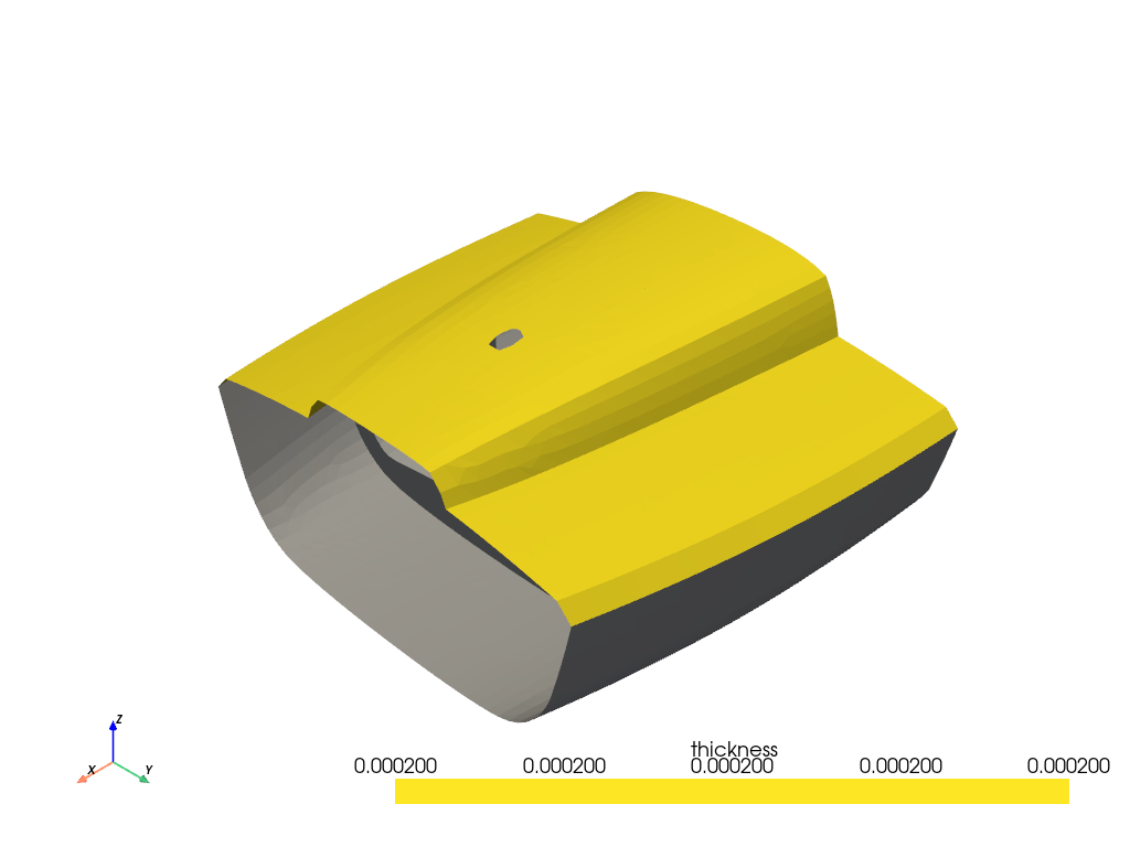
Show the thickness of one of the plies.
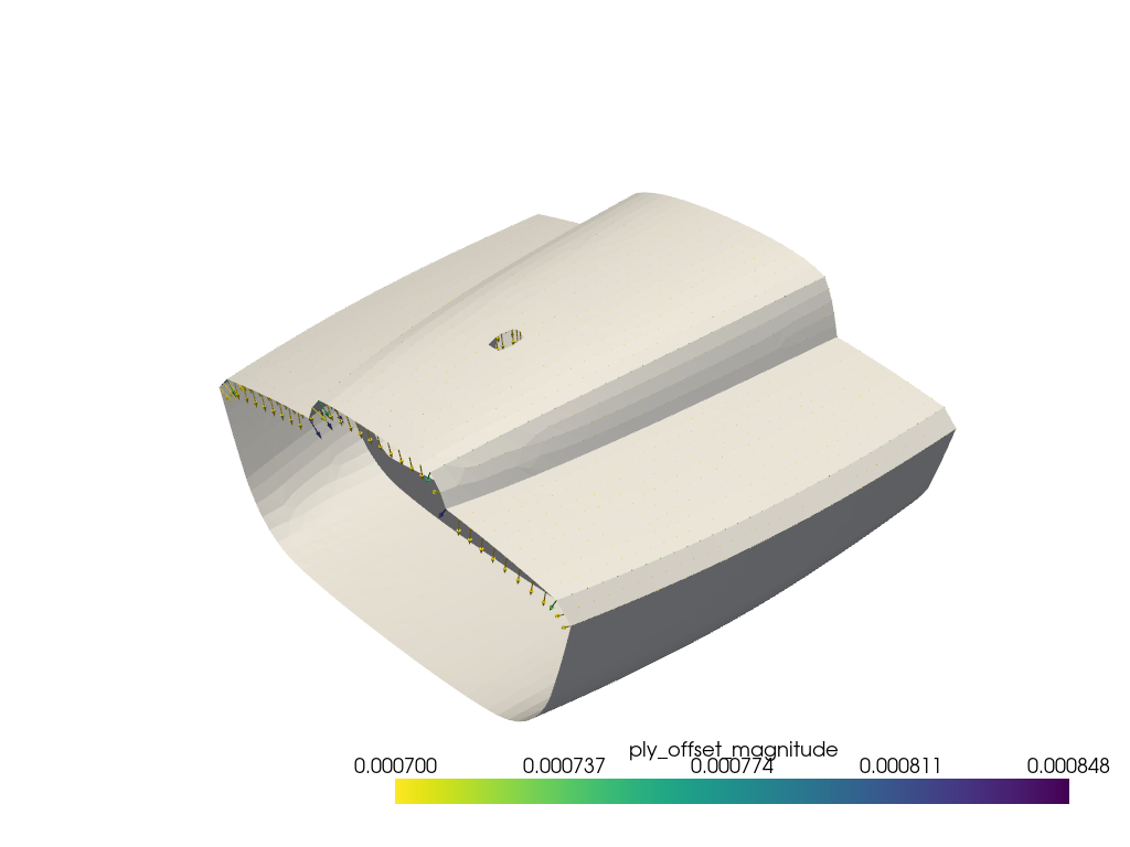
Show the ply offsets that are scaled by a factor of 200.
plotter = pyvista.Plotter()
plotter.add_mesh(model.mesh.to_pyvista(), color="white")
ply_offset = modeling_ply.nodal_data.ply_offset
assert ply_offset is not None
plotter.add_mesh(
    ply_offset.get_pyvista_glyphs(mesh=model.mesh, factor=200),
)
plotter.show()
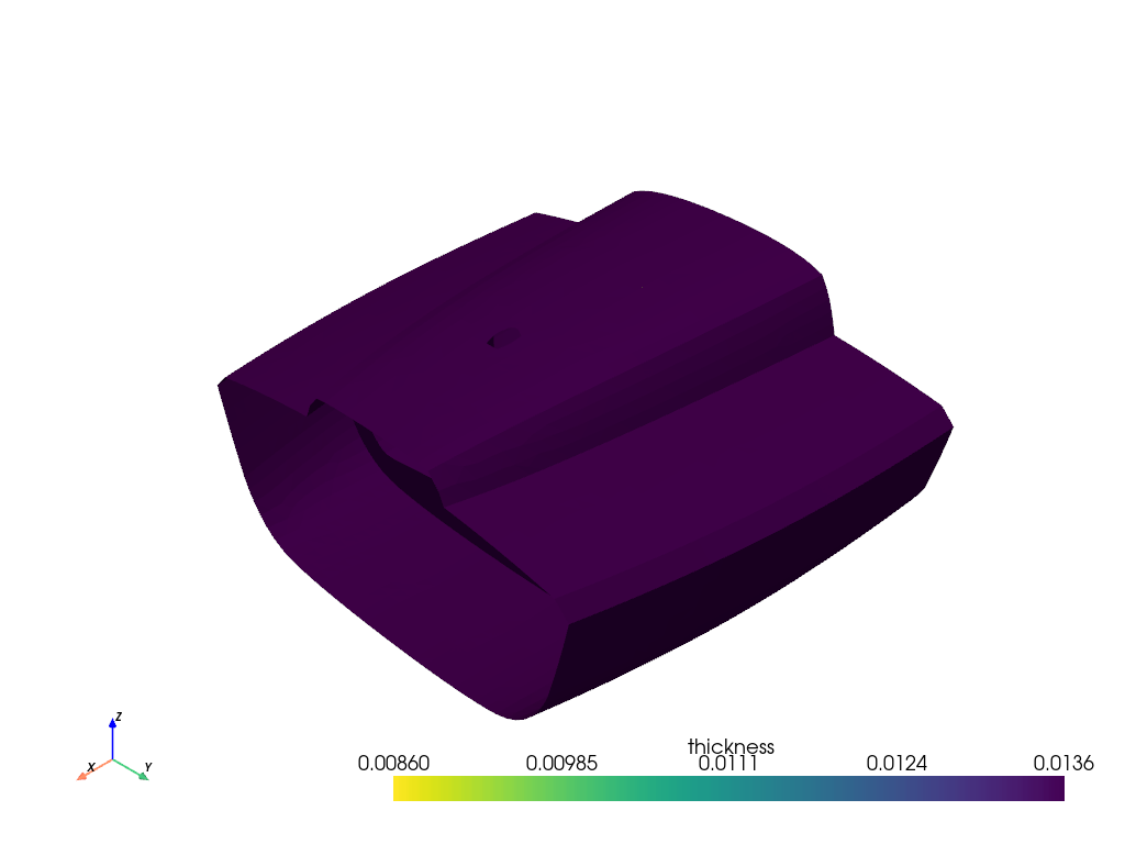
Show the thickness of the entire lay-up.
Write out ACP Model#
acph5_filename = "class40.acph5"
cdb_filename_out = "class40_analysis_model.cdb"
composite_definition_h5_filename = "ACPCompositeDefinitions.h5"
matml_filename = "materials.xml"
Update and save the ACP model.
model.update()
model.save(working_dir_path / acph5_filename, save_cache=True)
Save the model as a CDB file for solving with PyMAPDL.
model.export_analysis_model(working_dir_path / cdb_filename_out)
# Export the shell lay-up and material file for PyDPF - Composites.
model.export_shell_composite_definitions(working_dir_path / composite_definition_h5_filename)
model.export_materials(working_dir_path / matml_filename)
Solve with PyMAPDL#
Import PyMAPDL and connect to its server.
from ansys.mapdl.core import launch_mapdl

mapdl = launch_mapdl()
mapdl.clear()
Load the CDB file into PyMAPDL.
mapdl.input(str(working_dir_path / cdb_filename_out))
'\n /INPUT FILE= LINE= 0\n ANSYS RELEASE 11.0 UP20070125 16:39:41 03/10/2009\n *****MAPDL VERIFICATION RUN ONLY*****\n DO NOT USE RESULTS FOR PRODUCTION\n\n ***** MAPDL ANALYSIS DEFINITION (PREP7) *****\n\n\n ***** ROUTINE COMPLETED ***** ELAPSED TIME = 0.000\n\n\n'
Solve the model.
mapdl.allsel()
mapdl.slashsolu()
mapdl.solve()
*****  MAPDL SOLVE    COMMAND  *****

 *** NOTE ***                            ELAPSED TIME =       0.000   TIME= 00:00:00
 There is no title defined for this analysis.

 *** SELECTION OF ELEMENT TECHNOLOGIES FOR APPLICABLE ELEMENTS ***
                ---GIVE SUGGESTIONS ONLY---

 ELEMENT TYPE         1 IS SHELL181. IT IS ASSOCIATED WITH ELASTOPLASTIC
 MATERIALS ONLY. KEYOPT(8) IS ALREADY SET AS SUGGESTED. KEYOPT(3)=2
 IS SUGGESTED FOR HIGHER ACCURACY OF MEMBRANE STRESSES; OTHERWISE,
 KEYOPT(3)=0 IS SUGGESTED.

 ELEMENT TYPE         2 IS BEAM188 . KEYOPT(1)=1 IS SUGGESTED FOR NON-CIRCULAR CROSS
 SECTIONS AND KEYOPT(3)=2 IS ALWAYS SUGGESTED.

 ELEMENT TYPE         2 IS BEAM188 . KEYOPT(15) IS ALREADY SET AS SUGGESTED.

 ELEMENT TYPE         3 IS SHELL181. IT IS ASSOCIATED WITH ELASTOPLASTIC
 MATERIALS ONLY. KEYOPT(8) IS ALREADY SET AS SUGGESTED. KEYOPT(3)=2
 IS SUGGESTED FOR HIGHER ACCURACY OF MEMBRANE STRESSES; OTHERWISE,
 KEYOPT(3)=0 IS SUGGESTED.


   *****MAPDL VERIFICATION RUN ONLY*****
     DO NOT USE RESULTS FOR PRODUCTION

                       S O L U T I O N   O P T I O N S

   PROBLEM DIMENSIONALITY. . . . . . . . . . . . .3-D
   DEGREES OF FREEDOM. . . . . . UX   UY   UZ   ROTX ROTY ROTZ
   ANALYSIS TYPE . . . . . . . . . . . . . . . . .STATIC (STEADY-STATE)
   GLOBALLY ASSEMBLED MATRIX . . . . . . . . . . .SYMMETRIC

 *** NOTE ***                            ELAPSED TIME =       0.000   TIME= 00:00:00
 Poisson's ratio PR input has been converted to NU input.

 *** NOTE ***                            ELAPSED TIME =       0.000   TIME= 00:00:00
 Present time 0 is less than or equal to the previous time.  Time will
 default to 1.

 *** NOTE ***                            ELAPSED TIME =       0.000   TIME= 00:00:00
 The conditions for direct assembly have been met.  No .emat or .erot
 files will be produced.

                      L O A D   S T E P   O P T I O N S

   LOAD STEP NUMBER. . . . . . . . . . . . . . . .     1
   TIME AT END OF THE LOAD STEP. . . . . . . . . .  1.0000
   NUMBER OF SUBSTEPS. . . . . . . . . . . . . . .     1
   STEP CHANGE BOUNDARY CONDITIONS . . . . . . . .    NO
   PRINT OUTPUT CONTROLS . . . . . . . . . . . . .NO PRINTOUT
   DATABASE OUTPUT CONTROLS. . . . . . . . . . . .ALL DATA WRITTEN
                                                  FOR THE LAST SUBSTEP


 *** NOTE ***                            ELAPSED TIME =       0.000   TIME= 00:00:00
 Predictor is ON by default for structural elements with rotational
 degrees of freedom.  Use the PRED,OFF command to turn the predictor
 OFF if it adversely affects the convergence.


                         ***********  PRECISE MASS SUMMARY  ***********

   TOTAL RIGID BODY MASS MATRIX ABOUT ORIGIN
               Translational mass               |   Coupled translational/rotational mass
         324.96       0.16229E-18   0.36852E-17 |   -0.69755E-17    211.44      -0.36088E-02
        0.18942E-18    324.96       0.25320E-17 |    -211.44       0.37627E-16   -2015.3
        0.36851E-17   0.25320E-17    324.96     |    0.36088E-02    2015.3      -0.30584E-16
     ------------------------------------------ | ------------------------------------------
                                                |         Rotational mass (inertia)
                                                |     759.66       0.20436E-01    1316.9
                                                |    0.20436E-01    13054.      -0.32469E-02
                                                |     1316.9      -0.32469E-02    13218.

   TOTAL MASS =  324.96
     The mass principal axes coincide with the global Cartesian axes

   CENTER OF MASS (X,Y,Z)=   -6.2017       0.11105E-04   0.65067

   TOTAL INERTIA ABOUT CENTER OF MASS
         622.08      -0.19444E-02    5.6093
       -0.19444E-02    418.20      -0.89877E-03
         5.6093      -0.89877E-03    719.59

   PRINCIPAL INERTIAS =    621.76        418.20        719.92
   ORIENTATION VECTORS OF THE INERTIA PRINCIPAL AXES IN GLOBAL CARTESIAN
     ( 0.998,-0.000,-0.057) ( 0.000, 1.000, 0.000) ( 0.057,-0.000, 0.998)


  *** MASS SUMMARY BY ELEMENT TYPE ***

  TYPE      MASS
     1   322.570
     2   1.65744
     3  0.729815

 Range of element maximum matrix coefficients in global coordinates
 Maximum = 104467551 at element 0.
 Minimum = 31671440.9 at element 0.

   *** ELEMENT MATRIX FORMULATION TIMES
     TYPE    NUMBER     ENAME   TOTAL ELAPSED   AVG ELAPSED

        1      3973  SHELL181          0.0000   0.000000000
        2        88   BEAM188          0.0000   0.000000000
        3        22  SHELL181          0.0000   0.000000000
 Elapsed Time at end of element matrix formulation = 0.

 SPARSE MATRIX DIRECT SOLVER.
  Number of equations =       24096,    Maximum wavefront =      0
  Memory available (MB) =    0.0    ,  Memory required (MB) =    0.0

 Sparse solver maximum pivot= 0 at node 0 .
 Sparse solver minimum pivot= 0 at node 0 .
 Sparse solver minimum pivot in absolute value= 0 at node 0 .

   *** ELEMENT RESULT CALCULATION TIMES
     TYPE    NUMBER     ENAME   TOTAL ELAPSED   AVG ELAPSED

        1      3973  SHELL181          0.0000   0.000000000
        2        88   BEAM188          0.0000   0.000000000
        3        22  SHELL181          0.0000   0.000000000

   *** NODAL LOAD CALCULATION TIMES
     TYPE    NUMBER     ENAME   TOTAL ELAPSED   AVG ELAPSED

        1      3973  SHELL181          0.0000   0.000000000
        2        88   BEAM188          0.0000   0.000000000
        3        22  SHELL181          0.0000   0.000000000
 *** LOAD STEP     1   SUBSTEP     1  COMPLETED.    CUM ITER =      1
 *** TIME =   1.00000         TIME INC =   1.00000      NEW TRIANG MATRIX
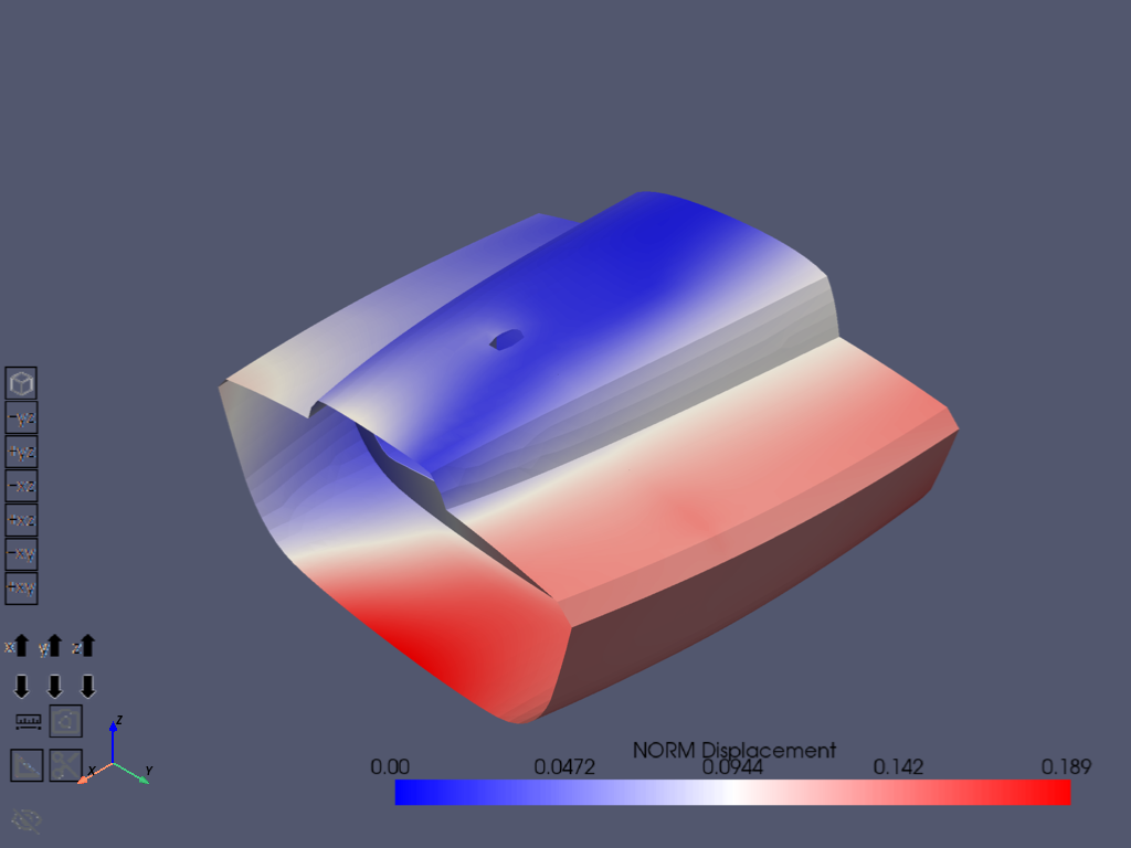
Show the displacements in postprocessing.
mapdl.post1()
mapdl.set("last")
mapdl.post_processing.plot_nodal_displacement(component="NORM")

# Download the RST file for further postprocessing.
rstfile_name = f"{mapdl.jobname}.rst"
mapdl.download(rstfile_name, working_dir_path)
[84, 89, 109]

['file.rst']
Postprocessing with PyDPF - Composites#
To postprocess the results, you must configure the imports, connect to the PyDPF - Composites server, and load its plugin.
from ansys.acp.core.dpf_integration_helpers import get_dpf_unit_system
from ansys.dpf.composites.composite_model import CompositeModel
from ansys.dpf.composites.constants import FailureOutput
from ansys.dpf.composites.data_sources import (
    CompositeDefinitionFiles,
    ContinuousFiberCompositesFiles,
)
from ansys.dpf.composites.failure_criteria import (
    CombinedFailureCriterion,
    CoreFailureCriterion,
    MaxStrainCriterion,
    MaxStressCriterion,
)
from ansys.dpf.composites.server_helpers import connect_to_or_start_server
Connect to the server. The connect_to_or_start_server function
automatically loads the composites plugin.
dpf_server = connect_to_or_start_server()
Specify the combined failure criterion.
max_strain = MaxStrainCriterion()
max_stress = MaxStressCriterion()
core_failure = CoreFailureCriterion()

cfc = CombinedFailureCriterion(
    name="Combined Failure Criterion",
    failure_criteria=[max_strain, max_stress, core_failure],
)
Create the composite model and configure its input.
composite_model = CompositeModel(
    composite_files=ContinuousFiberCompositesFiles(
        rst=working_dir_path / rstfile_name,
        composite={
            "shell": CompositeDefinitionFiles(
                definition=working_dir_path / composite_definition_h5_filename
            ),
        },
        engineering_data=working_dir_path / matml_filename,
    ),
    default_unit_system=get_dpf_unit_system(model.unit_system),
    server=dpf_server,
)
Evaluate the failure criteria.
output_all_elements = composite_model.evaluate_failure_criteria(cfc)
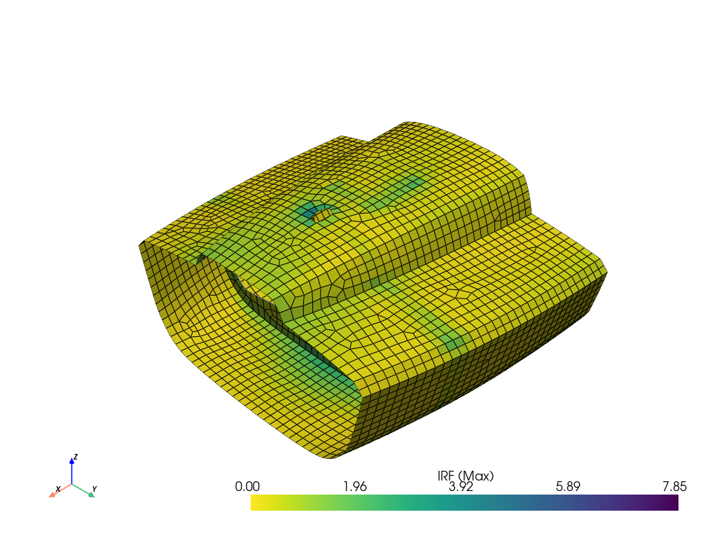
Query and plot the results.
irf_field = output_all_elements.get_field({"failure_label": FailureOutput.FAILURE_VALUE})
irf_field.plot()

# Close MAPDL instance
mapdl.exit()
Total running time of the script: (0 minutes 37.060 seconds)